

278
8. Applications of Groundwater Quality Models
on decision variables, h; may be represented as h;{P I , P 2 , ••• , Pm), i = 1, 2, ... ,
m. In Eq. (8.3.3), <5{.) is the Dirac-<5 function, {x;, yJ the coordinates of
pumping weIl Wi, (rd the constant head boundary and (r 2 ) the no-flow
boundary. The steady state heads should satisfy the following constraint in
order to limit excessive drawdown in the weIls:
(8.3.4)
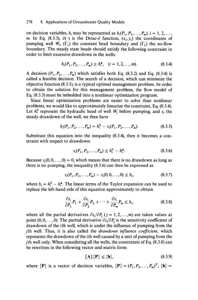
Adecision (PI' P2 , ••• , Pm) which satisfies both Eq. (8.3.2) and Eq. (8.3.4) is
called a feasible decision. The search of adecision, which can minimize the
objective function (8.3.1), is a typical optimal management problem. In order
to obtain the solution for this management problem, the flow model of
Eq. (8.3.3) must be imbedded into a nonlinear optimization program.
Since linear optimization problems are easier to solve than nonlinear
problems, we would like to approximately linearize the constraint, Eq. (8.3.4).
Let h? represent the hydraulic head of weIl Wi before pumping, and S; the
steady drawdown of the weIl, we then have
(8.3.5)
Substitute this equation into the inequality (8.3.4), then it becomes a constraint with respect to drawdown:
(8.3.6)
Because s;(O, 0, ... ,0) = 0, which means that there is no drawdown as long as
there is no pumping, the inequality (8.3.6) can then be expressed as
(8.3.7)
where b; = h? - hr. The linear terms of the Taylor expansion can be used to
replace the left-hand side of this equation approximately to obtain
(8.3.8)
where all the partial derivatives f}s;/f}~ (j = 1,2, ... , m) are taken values at
point (0,0, ... ,0). The partial derivative f}sJf}~ is the sensitivity coefficient of
drawdown of the ith weIl, which is under the influence of pumping from the
jth weIl. Thus, it is also called the drawdown irifluence coefficient, which
represents the drawdown ofthe ith weIl caused by a unit ofpumping from the
jth weIl only. When considering all the weIls, the constraints of Eq. (8.3.8) can
be rewritten in the following vector and matrix form:
[AJ {P} ~ {b},
(8.3.9)
where {P} is a vector of decision variables, {P} = (PI,P2, ... ,Pm )T; {b} =
8. Applications of Groundwater Quality Models
on decision variables, h; may be represented as h;{P I , P 2 , ••• , Pm), i = 1, 2, ... ,
m. In Eq. (8.3.3), <5{.) is the Dirac-<5 function, {x;, yJ the coordinates of
pumping weIl Wi, (rd the constant head boundary and (r 2 ) the no-flow
boundary. The steady state heads should satisfy the following constraint in
order to limit excessive drawdown in the weIls:
(8.3.4)
Adecision (PI' P2 , ••• , Pm) which satisfies both Eq. (8.3.2) and Eq. (8.3.4) is
called a feasible decision. The search of adecision, which can minimize the
objective function (8.3.1), is a typical optimal management problem. In order
to obtain the solution for this management problem, the flow model of
Eq. (8.3.3) must be imbedded into a nonlinear optimization program.
Since linear optimization problems are easier to solve than nonlinear
problems, we would like to approximately linearize the constraint, Eq. (8.3.4).
Let h? represent the hydraulic head of weIl Wi before pumping, and S; the
steady drawdown of the weIl, we then have
(8.3.5)
Substitute this equation into the inequality (8.3.4), then it becomes a constraint with respect to drawdown:
(8.3.6)
Because s;(O, 0, ... ,0) = 0, which means that there is no drawdown as long as
there is no pumping, the inequality (8.3.6) can then be expressed as
(8.3.7)
where b; = h? - hr. The linear terms of the Taylor expansion can be used to
replace the left-hand side of this equation approximately to obtain
(8.3.8)
where all the partial derivatives f}s;/f}~ (j = 1,2, ... , m) are taken values at
point (0,0, ... ,0). The partial derivative f}sJf}~ is the sensitivity coefficient of
drawdown of the ith weIl, which is under the influence of pumping from the
jth weIl. Thus, it is also called the drawdown irifluence coefficient, which
represents the drawdown ofthe ith weIl caused by a unit ofpumping from the
jth weIl only. When considering all the weIls, the constraints of Eq. (8.3.8) can
be rewritten in the following vector and matrix form:
[AJ {P} ~ {b},
(8.3.9)
where {P} is a vector of decision variables, {P} = (PI,P2, ... ,Pm )T; {b} =