

8.3. Groundwater Quality Management Models
277
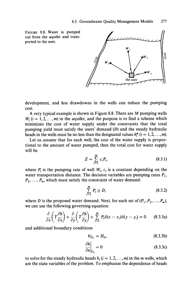
FIGURE 8.8. Water is pumped
out from the aquifer and transported to the user.
....
'1)
.~
development, and less drawdowns in the weHs can reduce the pumping
cost.
A very typical example is shown in Figure 8.8. There are M pumping weHs
W; (i = 1,2, ... , m) in the aquifer, and the purpose is to find a scheme wh ich
minimizes the cost of water supply under the constraints that the total
pumping yield must satisfy the users' demand (D) and the steady hydraulic
heads in the weHs must be no less than the designated values ht (i = 1,2, ... , m).
Let us assume that for each weH, the cost of the water supply is proportional to the amount of water pumped, then the total cost for water supply
will be
m
Z= L CiPi,
(8.3.1 )
i=1
where Pi is the pumping rate of weH W;, Ci is a constant depending on the
water transportation distance. The decision variables are pumping rates PI'
P2 , ••• , Pm' which must satisfy the constraint of water demand:
m
L Pi~D,
(8.3.2)
i=1
where D is the proposed water demand. Next, for each set of (PI' P 2 , . .. , Pm)'
we can use the following governing equation:
a~( T:~) + ;y( T:~) + i~ PJj(X - x i )c5(y - yJ = 0 (8.3.3a)
and additional boundary conditions
hlr ! = Ho,
(8.3.3b)
ahl = 0
an r 2
(8.3.3c)
to solve for the steady hydraulic heads h i (i = 1,2, ... , m) in the m weHs, which
are the state variables of the problem. To emphasize the dependence of heads
277
FIGURE 8.8. Water is pumped
out from the aquifer and transported to the user.
....
'1)
.~
development, and less drawdowns in the weHs can reduce the pumping
cost.
A very typical example is shown in Figure 8.8. There are M pumping weHs
W; (i = 1,2, ... , m) in the aquifer, and the purpose is to find a scheme wh ich
minimizes the cost of water supply under the constraints that the total
pumping yield must satisfy the users' demand (D) and the steady hydraulic
heads in the weHs must be no less than the designated values ht (i = 1,2, ... , m).
Let us assume that for each weH, the cost of the water supply is proportional to the amount of water pumped, then the total cost for water supply
will be
m
Z= L CiPi,
(8.3.1 )
i=1
where Pi is the pumping rate of weH W;, Ci is a constant depending on the
water transportation distance. The decision variables are pumping rates PI'
P2 , ••• , Pm' which must satisfy the constraint of water demand:
m
L Pi~D,
(8.3.2)
i=1
where D is the proposed water demand. Next, for each set of (PI' P 2 , . .. , Pm)'
we can use the following governing equation:
a~( T:~) + ;y( T:~) + i~ PJj(X - x i )c5(y - yJ = 0 (8.3.3a)
and additional boundary conditions
hlr ! = Ho,
(8.3.3b)
ahl = 0
an r 2
(8.3.3c)
to solve for the steady hydraulic heads h i (i = 1,2, ... , m) in the m weHs, which
are the state variables of the problem. To emphasize the dependence of heads