

8.3. Groundwater Quality Management Models
275
to obtain a set of ordinary differential equations,
dC
[A]C + [B]Tt + F = 0,
(8.2.50)
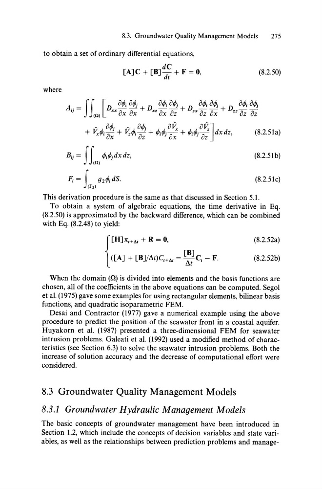
where
(8.2.51b)
(8.2.51c)
This derivation procedure is the same as that discussed in Section 5.1.
To obtain a system of algebraic equations, the time derivative in Eq.
(8.2.50) is approximated by the back ward difference, which can be combined
with Eq. (8.2.48) to yield:
{
[H] TCtHt + R = 0,
[B]
([A] + [B]/At)CtH, = TtCt - F.
(8.2.52a)
(8.2.52b)
When the domain (0) is divided into elements and the basis functions are
chosen, aIl of the coefficients in the above equations can be computed. Segol
et al. (1975) gave some examples for using rectangular elements, bilinear basis
functions, and quadratic isoparametric FEM.
Desai and Contractor (1977) gave a numerical example using the above
procedure to predict the position of the seawater front in a coastal aquifer.
Huyakorn et al. (1987) presented a three-dimensional FEM for seawater
intrusion problems. Galeati et al. (1992) used a modified method of characteristics (see Section 6.3) to solve the seawater intrusion problems. Both the
increase of solution accuracy and the decrease of computational effort were
considered.
8.3 Groundwater Quality Management Models
8.3.1 Groundwater Hydraulic Management Models
The basic concepts of groundwater management have been introduced in
Section 1.2, which include the concepts of decision variables and state variables, as weIl as the relationships between prediction problems and manage-
275
to obtain a set of ordinary differential equations,
dC
[A]C + [B]Tt + F = 0,
(8.2.50)
where
(8.2.51b)
(8.2.51c)
This derivation procedure is the same as that discussed in Section 5.1.
To obtain a system of algebraic equations, the time derivative in Eq.
(8.2.50) is approximated by the back ward difference, which can be combined
with Eq. (8.2.48) to yield:
{
[H] TCtHt + R = 0,
[B]
([A] + [B]/At)CtH, = TtCt - F.
(8.2.52a)
(8.2.52b)
When the domain (0) is divided into elements and the basis functions are
chosen, aIl of the coefficients in the above equations can be computed. Segol
et al. (1975) gave some examples for using rectangular elements, bilinear basis
functions, and quadratic isoparametric FEM.
Desai and Contractor (1977) gave a numerical example using the above
procedure to predict the position of the seawater front in a coastal aquifer.
Huyakorn et al. (1987) presented a three-dimensional FEM for seawater
intrusion problems. Galeati et al. (1992) used a modified method of characteristics (see Section 6.3) to solve the seawater intrusion problems. Both the
increase of solution accuracy and the decrease of computational effort were
considered.
8.3 Groundwater Quality Management Models
8.3.1 Groundwater Hydraulic Management Models
The basic concepts of groundwater management have been introduced in
Section 1.2, which include the concepts of decision variables and state variables, as weIl as the relationships between prediction problems and manage-