

7.3. Coupled Inverse Problems of Groundwater Flow and Mass Transport
233
All parameters p satisfying the condition in Eq. (7.3.50) form a subset ofthe
admissible set which is named the predictive equivalent set of j). Our question
is: can we design an experiment, so that when we use the results of the
experiment to solve the inverse problem, the parameters obtained will certainly belong to the predictive equivalent set of j)? If the answer is positive,
parameter j) is said to be prediction equivalence identifiable. By comparing it
with the classical definition of identifiability mentioned above, we can see
that this kind of extended identifiability does not require the uniqueness
either for the inverse problem or for the optimization problem (7.3.12). The
major advantage of prediction equivalence identifiability is that it may be
satisfied in practice by limited quantity and quality of observed data.
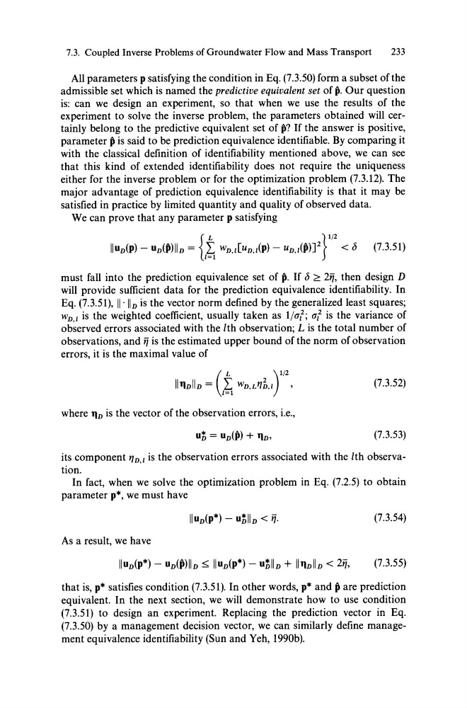
We can prove that any parameter p satisfying
(7.3.51)
must fall into the prediction equivalence set of j). If f> ~ 2ij, then design D
will provide sufficient data for the prediction equivalence identifiability. In
Eq. (7.3.51), 11' liD is the vector norm defined by the generalized least squares;
WD,1 is the weighted coefficient, usually taken as l/a?; a? is the variance of
observed errors associated with the lth observation; L is the total number of
observations, and ij is the estimated upper bound of the norm of observation
errors, it is the maximal value of
( L
)1/2
IlllDIlD = l~ WD ,L1J1.1 ,
(7.3.52)
where llD is the vector of the observation errors, i.e.,
(7.3.53)
its component 1JD,1 is the observation errors associated with the lth observation.
In fact, when we solve the optimization problem in Eq. (7.2.5) to obtain
parameter p*, we must have
(7.3.54)
As a result, we have
(7.3.55)
that is, p* satisfies condition (7.3.51). In other words, p* and j) are prediction
equivalent. In the next section, we will demonstrate how to use condition
(7.3.51) to design an experiment. Replacing the prediction vector in Eq.
(7.3.50) by a management decision vector, we can similarly define management equivalence identifiability (Sun and Yeh, 1990b).
233
All parameters p satisfying the condition in Eq. (7.3.50) form a subset ofthe
admissible set which is named the predictive equivalent set of j). Our question
is: can we design an experiment, so that when we use the results of the
experiment to solve the inverse problem, the parameters obtained will certainly belong to the predictive equivalent set of j)? If the answer is positive,
parameter j) is said to be prediction equivalence identifiable. By comparing it
with the classical definition of identifiability mentioned above, we can see
that this kind of extended identifiability does not require the uniqueness
either for the inverse problem or for the optimization problem (7.3.12). The
major advantage of prediction equivalence identifiability is that it may be
satisfied in practice by limited quantity and quality of observed data.
We can prove that any parameter p satisfying
(7.3.51)
must fall into the prediction equivalence set of j). If f> ~ 2ij, then design D
will provide sufficient data for the prediction equivalence identifiability. In
Eq. (7.3.51), 11' liD is the vector norm defined by the generalized least squares;
WD,1 is the weighted coefficient, usually taken as l/a?; a? is the variance of
observed errors associated with the lth observation; L is the total number of
observations, and ij is the estimated upper bound of the norm of observation
errors, it is the maximal value of
( L
)1/2
IlllDIlD = l~ WD ,L1J1.1 ,
(7.3.52)
where llD is the vector of the observation errors, i.e.,
(7.3.53)
its component 1JD,1 is the observation errors associated with the lth observation.
In fact, when we solve the optimization problem in Eq. (7.2.5) to obtain
parameter p*, we must have
(7.3.54)
As a result, we have
(7.3.55)
that is, p* satisfies condition (7.3.51). In other words, p* and j) are prediction
equivalent. In the next section, we will demonstrate how to use condition
(7.3.51) to design an experiment. Replacing the prediction vector in Eq.
(7.3.50) by a management decision vector, we can similarly define management equivalence identifiability (Sun and Yeh, 1990b).