

232
7. Mathematical Models of Groundwater Quality
always exist in practice, if a minor change in the observations causes a great
change in the parameter to be determined, then we cannot find the true
parameter either. This is the problem of instability.
Some simple examples of non-uniqueness and instability in the solution
of the inverse problem of groundwater flow are given by Neuman (1973),
Chavent (1979), Sun (1981) and Sun (1994). When solving the inverse problem of groundwater quality, the non-uniqueness resulting from the coexistence of advection and dispersion terms may become very significant.
An essential problem in parameter identification is the identifiability problem. The classical definition of identifiability (Kitamura and Nakagiri, 1977)
requires that the unknown parameter be uniquely determined by the observation data obtained from an experimental design. According to this definition, the value of the unknown parameter and the set of observations must
correspond to each other one by one. Of course, it is impossible to meet
this demand in practice.
Chavent (1979) put forward another concept of identifiability, the Least
Squares ldentifiability. It only requires that the optimization problem in Eq.
(7.2.5) have a unique solution, and this solution continuously depend on the
observation data. This definition allows the existence of observation errors.
However, it is still difficult to satisfy in practice. Yeh and Sun (1984) suggested a concept, b-identifiability, which only requires that the predicted
results not greatly deviate from the real results when the identified parameters is used for a prediction purpose. Various definitions of identifiability
were reviewed by Chavent (1987). Sun and Yeh (1990b) presented the Prediction Equivalence ldentifiability and Management Equivalence ldentifiability
for general coupled problems. Based on these ideas, hydrogeologists can
design experiments and identify parameters in accordance with the accuracy demanded by the manager, so as to guarantee the reliability of model
applications.
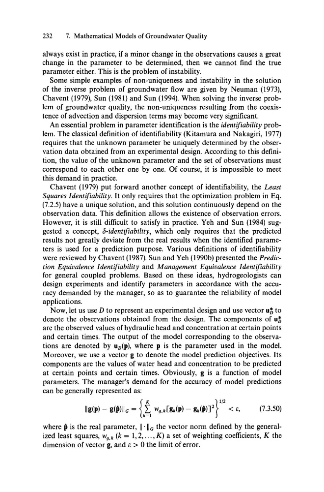
Now, let us use D to represent an experimental design and use vector u1) to
denote the observations obtained from the design. The components of u1)
are the observed values ofhydraulic head and concentration at certain points
and certain times. The output of the model corresponding to the observations are denoted by uD(p), where p is the parameter used in the model.
Moreover, we use a vector g to denote the model prediction objectives. Its
components are the values of water head and concentration to be predicted
at certain points and certain times. Obviously, g is a function of model
parameters. The manager's demand for the accuracy of model predictions
can be generally represented as:
{
K
} 1/2
IIg(p) - g(~)IIG = kf: 1 W9,k[gk(P) - gk(~)]2
< 8,
(7.3.50)
where ß is the real parameter, 11' 11 G the vector norm defined by the generalized least squares, Wg,k (k = 1,2, ... , K) a set of weighting coefficients, K the
dimension of vector g, and 8 > 0 the limit of error.
7. Mathematical Models of Groundwater Quality
always exist in practice, if a minor change in the observations causes a great
change in the parameter to be determined, then we cannot find the true
parameter either. This is the problem of instability.
Some simple examples of non-uniqueness and instability in the solution
of the inverse problem of groundwater flow are given by Neuman (1973),
Chavent (1979), Sun (1981) and Sun (1994). When solving the inverse problem of groundwater quality, the non-uniqueness resulting from the coexistence of advection and dispersion terms may become very significant.
An essential problem in parameter identification is the identifiability problem. The classical definition of identifiability (Kitamura and Nakagiri, 1977)
requires that the unknown parameter be uniquely determined by the observation data obtained from an experimental design. According to this definition, the value of the unknown parameter and the set of observations must
correspond to each other one by one. Of course, it is impossible to meet
this demand in practice.
Chavent (1979) put forward another concept of identifiability, the Least
Squares ldentifiability. It only requires that the optimization problem in Eq.
(7.2.5) have a unique solution, and this solution continuously depend on the
observation data. This definition allows the existence of observation errors.
However, it is still difficult to satisfy in practice. Yeh and Sun (1984) suggested a concept, b-identifiability, which only requires that the predicted
results not greatly deviate from the real results when the identified parameters is used for a prediction purpose. Various definitions of identifiability
were reviewed by Chavent (1987). Sun and Yeh (1990b) presented the Prediction Equivalence ldentifiability and Management Equivalence ldentifiability
for general coupled problems. Based on these ideas, hydrogeologists can
design experiments and identify parameters in accordance with the accuracy demanded by the manager, so as to guarantee the reliability of model
applications.
Now, let us use D to represent an experimental design and use vector u1) to
denote the observations obtained from the design. The components of u1)
are the observed values ofhydraulic head and concentration at certain points
and certain times. The output of the model corresponding to the observations are denoted by uD(p), where p is the parameter used in the model.
Moreover, we use a vector g to denote the model prediction objectives. Its
components are the values of water head and concentration to be predicted
at certain points and certain times. Obviously, g is a function of model
parameters. The manager's demand for the accuracy of model predictions
can be generally represented as:
{
K
} 1/2
IIg(p) - g(~)IIG = kf: 1 W9,k[gk(P) - gk(~)]2
< 8,
(7.3.50)
where ß is the real parameter, 11' 11 G the vector norm defined by the generalized least squares, Wg,k (k = 1,2, ... , K) a set of weighting coefficients, K the
dimension of vector g, and 8 > 0 the limit of error.