

230
7. Mathematical Models of Groundwater Quality
Summarily, there are two problems here: the original coupled problem
defined by Eqs. (7.3.1) to (7.3.5) and its adjoint problem. The governing
equations of the latter are Eqs. (7.3.41) and (7.3.42), where the final and
boundary conditions for tP1 are defined by Eqs. (7.3.29), (7.3.30), and (7.3.40),
and those for tP2' by Eqs. (7.3.33), (7.3.34), and (7.3.35). The distributions of
hand C can be determined by solving original coupled problem, and the
distributions of tP1 and tP2 can be determined by solving the adjoint problem.
As a result, integrand (7.3.43) can be calculated.
If the variable substitution, 't' = T - t, is made in the adjoint problem, Eqs.
(7.3.41) and (7.3.42) will become identical to the original coupled problem in
form. The final condition will turn into the initial condition. Hence, we need
only to slightly modify the subprogram for solving hand C, which can then
be used for solving tP1 and tP2' The detailed solution procedure and numerical
examples may be found from Sun and Yeh (1990a). Next, let us demonstrate
the usage of Eq. (7.3.43), the variation of the objective function. Assume
that K is parameterized by the zonation method, that is, the whole domain
(n) is divided into m subdomains (nd, (n2 ), ... , (nm)' K is a constant
in each subdomain. The unknown parameter vector now becomes K =
(K 1 ,K 2 , ... ,K m f. To calculate the gradient (7.3.14), the function to be
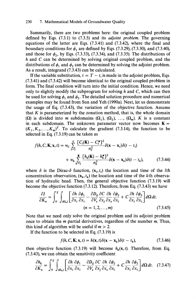
selected in Eq. (7.3.19) can be taken as
L [C,(K) - C,*J2
f(h, C, K; x, t) = Wc L
2
b(X - x,)b(t - t,)
'=1
Uc
(7.3.44)
where b is the Dirac-b function, (x" t,) the location and time of the lth
concentration observation, (x k , t k ) the location and time of the kth observation of hydraulic head. Then, the general objective function (7.3.19) will
become the objective function (7.3.12). Therefore, from Eq. (7.3.43) we have
~ = fT f [8h 8tP1 _ 8Dij 8C 8h 8tP2 + C 8h 8tP2Jdndt.
8Kn Jo JOn) 8xi 8Xi 8V. 8xj 8xs 8xi 8Xi 8Xi
(n = 1,2, ... , m)
(7.3.45)
Note that we need only solve the original problem and its adjoint problem
once to obtain the m partial derivatives, regardless of the number m. Thus,
this kind of algorithm will be useful if m > 2.
If the function to be selected in Eq. (7.3.19) is
f(h, C, K; x, t) = h(x, t)<5(x - x k )<5(t - t k ),
(7.3.46)
then objective function (7.3.19) will become hk(x, t). Therefore, from Eq.
(7.3.43), we can obtain the sensitivity coefficient
8hk = f T f [8h 8tP1 _ 8Dij 8C ~ 8tP2 + C 8h 8tP2] dn dt. (7.3.47)
8Kn Jo J(On) 8Xi 8xi 8V. 8xj 8xs 8Xi 8xi 8Xi
7. Mathematical Models of Groundwater Quality
Summarily, there are two problems here: the original coupled problem
defined by Eqs. (7.3.1) to (7.3.5) and its adjoint problem. The governing
equations of the latter are Eqs. (7.3.41) and (7.3.42), where the final and
boundary conditions for tP1 are defined by Eqs. (7.3.29), (7.3.30), and (7.3.40),
and those for tP2' by Eqs. (7.3.33), (7.3.34), and (7.3.35). The distributions of
hand C can be determined by solving original coupled problem, and the
distributions of tP1 and tP2 can be determined by solving the adjoint problem.
As a result, integrand (7.3.43) can be calculated.
If the variable substitution, 't' = T - t, is made in the adjoint problem, Eqs.
(7.3.41) and (7.3.42) will become identical to the original coupled problem in
form. The final condition will turn into the initial condition. Hence, we need
only to slightly modify the subprogram for solving hand C, which can then
be used for solving tP1 and tP2' The detailed solution procedure and numerical
examples may be found from Sun and Yeh (1990a). Next, let us demonstrate
the usage of Eq. (7.3.43), the variation of the objective function. Assume
that K is parameterized by the zonation method, that is, the whole domain
(n) is divided into m subdomains (nd, (n2 ), ... , (nm)' K is a constant
in each subdomain. The unknown parameter vector now becomes K =
(K 1 ,K 2 , ... ,K m f. To calculate the gradient (7.3.14), the function to be
selected in Eq. (7.3.19) can be taken as
L [C,(K) - C,*J2
f(h, C, K; x, t) = Wc L
2
b(X - x,)b(t - t,)
'=1
Uc
(7.3.44)
where b is the Dirac-b function, (x" t,) the location and time of the lth
concentration observation, (x k , t k ) the location and time of the kth observation of hydraulic head. Then, the general objective function (7.3.19) will
become the objective function (7.3.12). Therefore, from Eq. (7.3.43) we have
~ = fT f [8h 8tP1 _ 8Dij 8C 8h 8tP2 + C 8h 8tP2Jdndt.
8Kn Jo JOn) 8xi 8Xi 8V. 8xj 8xs 8xi 8Xi 8Xi
(n = 1,2, ... , m)
(7.3.45)
Note that we need only solve the original problem and its adjoint problem
once to obtain the m partial derivatives, regardless of the number m. Thus,
this kind of algorithm will be useful if m > 2.
If the function to be selected in Eq. (7.3.19) is
f(h, C, K; x, t) = h(x, t)<5(x - x k )<5(t - t k ),
(7.3.46)
then objective function (7.3.19) will become hk(x, t). Therefore, from Eq.
(7.3.43), we can obtain the sensitivity coefficient
8hk = f T f [8h 8tP1 _ 8Dij 8C ~ 8tP2 + C 8h 8tP2] dn dt. (7.3.47)
8Kn Jo J(On) 8Xi 8xi 8V. 8xj 8xs 8Xi 8xi 8Xi