

7.3. Coupled Inverse Problems of Groundwater Flow and Mass Transport
227
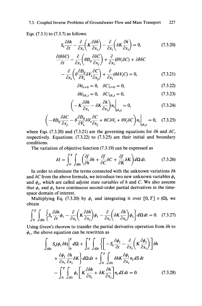
Eqs. (7.3.1) to (7.3.7) as folIows:
Ss obh _ ~(KObh) _ ~(bK Oh) = 0,
(7.3.20)
ot oXi oX i oX i oXi
(7.3.21)
(7.3.22)
(7.3.23)
(7.3.24)
(7.3.25)
where Eqs. (7.3.20) and (7.3.21) are the governing equations for bh and bC,
respectively. Equations. (7.3.22) to (7.3.25) are their initial and boundary
conditions.
The variation of objective function (7.3.19) can be expressed as
M = LT Ll ) (~ bh + :~bC + :~bK )dQdt. (7.3.26)
In order to eliminate the terms connected with the unknown variations bh
and bC from the above formula, we introduce two new unknown variables rP1
and rP2' which are called adjoint state variables of hand C. We also assume
that 1>1 and 1>2 have continuous second-order partial derivatives in the timespace domain of interest.
Multiplying Eq. (7.3.20) by rP1 and integrating it over [0, T] x (Q), we
obtain
LT Ll ) {Ss O:t h rP1 - O~i (K~~~)rP1 - O~i (bK ::)rP1 }dQdt = 0. (7.3.27)
Using Green's theorem to transfer the partial derivative operation from bh to
rP1' the above equation can be rewritten as
i SS(rP1bh)IT dQ + fT i {[-Ss a: 1 - -aa (K a
a rP1 )Jbh
(Q)
0
0
(Q)
ut
Xi
Xi
+ ~rP1 a oh bK} dQ dt + f Ti bhK aa rP1 ni dS dt
uXi Xi
0
(S)
Xi
f T i
[abh
OhJ
-
rP1 K- a + bK-a nidSdt = 0.
o (S)
Xi
Xi
(7.3.28)
227
Eqs. (7.3.1) to (7.3.7) as folIows:
Ss obh _ ~(KObh) _ ~(bK Oh) = 0,
(7.3.20)
ot oXi oX i oX i oXi
(7.3.21)
(7.3.22)
(7.3.23)
(7.3.24)
(7.3.25)
where Eqs. (7.3.20) and (7.3.21) are the governing equations for bh and bC,
respectively. Equations. (7.3.22) to (7.3.25) are their initial and boundary
conditions.
The variation of objective function (7.3.19) can be expressed as
M = LT Ll ) (~ bh + :~bC + :~bK )dQdt. (7.3.26)
In order to eliminate the terms connected with the unknown variations bh
and bC from the above formula, we introduce two new unknown variables rP1
and rP2' which are called adjoint state variables of hand C. We also assume
that 1>1 and 1>2 have continuous second-order partial derivatives in the timespace domain of interest.
Multiplying Eq. (7.3.20) by rP1 and integrating it over [0, T] x (Q), we
obtain
LT Ll ) {Ss O:t h rP1 - O~i (K~~~)rP1 - O~i (bK ::)rP1 }dQdt = 0. (7.3.27)
Using Green's theorem to transfer the partial derivative operation from bh to
rP1' the above equation can be rewritten as
i SS(rP1bh)IT dQ + fT i {[-Ss a: 1 - -aa (K a
a rP1 )Jbh
(Q)
0
0
(Q)
ut
Xi
Xi
+ ~rP1 a oh bK} dQ dt + f Ti bhK aa rP1 ni dS dt
uXi Xi
0
(S)
Xi
f T i
[abh
OhJ
-
rP1 K- a + bK-a nidSdt = 0.
o (S)
Xi
Xi
(7.3.28)