

7.3. Coupled Inverse Problems of Groundwater Flow and Mass Transport
225
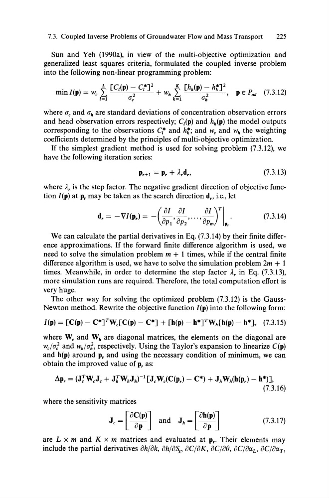
Sun and Yeh (1990a), in view of the multi-objective optimization and
generalized least squares criteria, formulated the coupled inverse problem
into the following non-linear programming problem:
. I() =
~ [C,(p) - C,*]2 + ~ [hk(p) - ht]2
P
(7312)
mm P We ~
2
Wh ~
2
, p E ad
••
'=1
(Tc
k=1
(Th
where (Tc and (Th are standard deviations of concentration observation errors
and head observation errors respectively; C,(p) and hk(p) the model outputs
corresponding to the observations C! and ht; and W e and Wh the weighting
coefficients determined by the principles of multi-objective optimization.
If the simplest gradient method is used for solving problem (7.3.12), we
have the following iteration series:
Pr+1 = Pr + Ard"
(7.3.13)
where Ar is the step factor. The negative gradient direction of objective functi on I(p) at Pr may be taken as the search direction d r , i.e., let
( iJI aJ
aJ )TI
dr = -V/(Pr) = - ~,~, ... ,~
.
UP1 UP2
UPm
'r
(7.3.14)
We can calculate the partial derivatives in Eq. (7.3.14) by their finite difference approximations. If the forward finite difference algorithm is used, we
need to solve the simulation problem m + 1 times, while if the central finite
difference algorithm is used, we have to solve the simulation problem 2m + 1
times. Meanwhile, in order to determine the step factor Ar in Eq. (7.3.13),
more simulation runs are required. Therefore, the total computation effort is
very huge.
The other way for solving the optimized problem (7.3.12) is the GaussNewton method. Rewrite the objective function I(p) into the following form:
I(p) = [C(p) - C*YWcEC(p) - C*] + [h(p) - h*YWh[h(p) - h*], (7.3.15)
where We and Wh are diagonal matrices, the elements on the diagonal are
wej(T; and Whj(T~, respectively. Using the Taylor's expansion to linearize C(p)
and h(p) around Pr and using the necessary condition of minimum, we can
obtain the improved value of Pr as:
L\Pr = (J~WeJe + JfWhJht 1 [Je We(C(Pr) - C*) + Jh Wh(h(Pr) - h*)],
(7.3.16)
where the sensitivity matrices
Je = [iJ~~P)J and Jh = [iJ~~)J
(7.3.17)
are L x m and K x m matrices and evaluated at Pr. Their elements may
include the partial derivatives iJhjiJk, iJhjiJS., iJCjiJK, iJCjoO, OCjOIXL' OCjOIXT'
225
Sun and Yeh (1990a), in view of the multi-objective optimization and
generalized least squares criteria, formulated the coupled inverse problem
into the following non-linear programming problem:
. I() =
~ [C,(p) - C,*]2 + ~ [hk(p) - ht]2
P
(7312)
mm P We ~
2
Wh ~
2
, p E ad
••
'=1
(Tc
k=1
(Th
where (Tc and (Th are standard deviations of concentration observation errors
and head observation errors respectively; C,(p) and hk(p) the model outputs
corresponding to the observations C! and ht; and W e and Wh the weighting
coefficients determined by the principles of multi-objective optimization.
If the simplest gradient method is used for solving problem (7.3.12), we
have the following iteration series:
Pr+1 = Pr + Ard"
(7.3.13)
where Ar is the step factor. The negative gradient direction of objective functi on I(p) at Pr may be taken as the search direction d r , i.e., let
( iJI aJ
aJ )TI
dr = -V/(Pr) = - ~,~, ... ,~
.
UP1 UP2
UPm
'r
(7.3.14)
We can calculate the partial derivatives in Eq. (7.3.14) by their finite difference approximations. If the forward finite difference algorithm is used, we
need to solve the simulation problem m + 1 times, while if the central finite
difference algorithm is used, we have to solve the simulation problem 2m + 1
times. Meanwhile, in order to determine the step factor Ar in Eq. (7.3.13),
more simulation runs are required. Therefore, the total computation effort is
very huge.
The other way for solving the optimized problem (7.3.12) is the GaussNewton method. Rewrite the objective function I(p) into the following form:
I(p) = [C(p) - C*YWcEC(p) - C*] + [h(p) - h*YWh[h(p) - h*], (7.3.15)
where We and Wh are diagonal matrices, the elements on the diagonal are
wej(T; and Whj(T~, respectively. Using the Taylor's expansion to linearize C(p)
and h(p) around Pr and using the necessary condition of minimum, we can
obtain the improved value of Pr as:
L\Pr = (J~WeJe + JfWhJht 1 [Je We(C(Pr) - C*) + Jh Wh(h(Pr) - h*)],
(7.3.16)
where the sensitivity matrices
Je = [iJ~~P)J and Jh = [iJ~~)J
(7.3.17)
are L x m and K x m matrices and evaluated at Pr. Their elements may
include the partial derivatives iJhjiJk, iJhjiJS., iJCjiJK, iJCjoO, OCjOIXL' OCjOIXT'