

224
7. Mathematical Models of Groundwater Quality
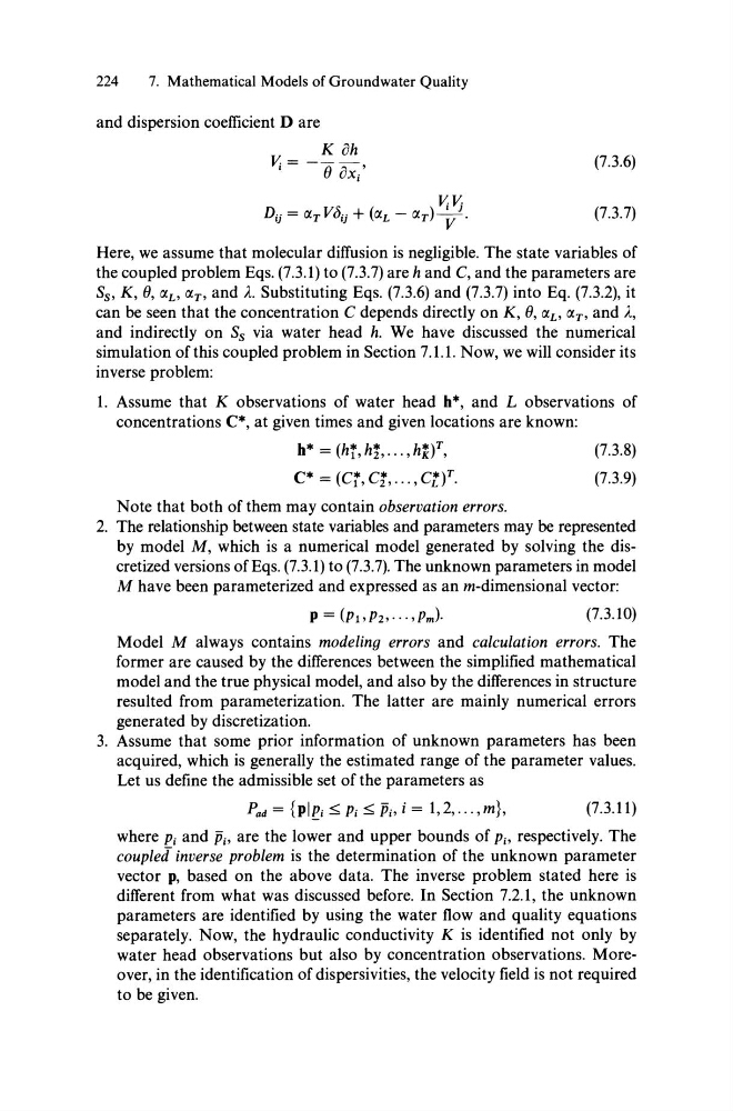
and dispersion coefficient D are
K oh
v,= - - -
I
(J ox/
v, v,
Dij = OC T V<5ij + (OCL - OCT) ~J.
(7.3.6)
(7.3.7)
Here, we assume that molecular diffusion is negligible. The state variables of
the coupled problem Eqs. (7.3.1) to (7.3.7) are hand C, and the parameters are
Ss, K, (J, OC L , OCT' and A.. Substituting Eqs. (7.3.6) and (7.3.7) into Eq. (7.3.2), it
can be seen that the concentration C depends directly on K, (J, oc L , oc T , and A.,
and indirectly on Ss via water head h. We have discussed the numerical
simulation ofthis coupled problem in Section 7.1.1. Now, we will consider its
inverse problem:
1. Assume that K observations of water head h*, and L observations of
concentrations C*, at given times and given locations are known:
h* = (hf,h!, ... ,h~V,
C* = (ct,C!, ... ,Ct)T.
Note that both of them may contain observation errors.
(7.3.8)
(7.3.9)
2. The relationship between state variables and parameters may be represented
by model M, which is a numerical model generated by solving the discretized versions ofEqs. (7.3.1) to (7.3.7). The unknown parameters in model
M have been parameterized and expressed as an m-dimensional vector:
(7.3.10)
Model M always contains modeling errors and calculation errors. The
former are caused by the differences between the simplified mathematical
model and the true physical model, and also by the differences in structure
resulted from parameterization. The latter are mainly numerical errors
generated by discretization.
3. Assume that some prior information of unknown parameters has been
acquired, which is generally the estimated range of the parameter values.
Let us define the admissible set of the parameters as
Pad = {plEi ~ Pi ~ Pi' i = 1,2, ... ,m},
(7.3.11)
where Pi and Pi' are the lower and upper bounds of Pi' respectively. The
coupled inverse problem is the determination of the unknown parameter
vector p, based on the above data. The inverse problem stated here is
different from what was discussed before. In Section 7.2.1, the unknown
parameters are identified by using the water flow and quality equations
separately. Now, the hydraulic conductivity K is identified not only by
water head observations but also by concentration observations. Moreover, in the identification of dispersivities, the velocity field is not required
to be given.
7. Mathematical Models of Groundwater Quality
and dispersion coefficient D are
K oh
v,= - - -
I
(J ox/
v, v,
Dij = OC T V<5ij + (OCL - OCT) ~J.
(7.3.6)
(7.3.7)
Here, we assume that molecular diffusion is negligible. The state variables of
the coupled problem Eqs. (7.3.1) to (7.3.7) are hand C, and the parameters are
Ss, K, (J, OC L , OCT' and A.. Substituting Eqs. (7.3.6) and (7.3.7) into Eq. (7.3.2), it
can be seen that the concentration C depends directly on K, (J, oc L , oc T , and A.,
and indirectly on Ss via water head h. We have discussed the numerical
simulation ofthis coupled problem in Section 7.1.1. Now, we will consider its
inverse problem:
1. Assume that K observations of water head h*, and L observations of
concentrations C*, at given times and given locations are known:
h* = (hf,h!, ... ,h~V,
C* = (ct,C!, ... ,Ct)T.
Note that both of them may contain observation errors.
(7.3.8)
(7.3.9)
2. The relationship between state variables and parameters may be represented
by model M, which is a numerical model generated by solving the discretized versions ofEqs. (7.3.1) to (7.3.7). The unknown parameters in model
M have been parameterized and expressed as an m-dimensional vector:
(7.3.10)
Model M always contains modeling errors and calculation errors. The
former are caused by the differences between the simplified mathematical
model and the true physical model, and also by the differences in structure
resulted from parameterization. The latter are mainly numerical errors
generated by discretization.
3. Assume that some prior information of unknown parameters has been
acquired, which is generally the estimated range of the parameter values.
Let us define the admissible set of the parameters as
Pad = {plEi ~ Pi ~ Pi' i = 1,2, ... ,m},
(7.3.11)
where Pi and Pi' are the lower and upper bounds of Pi' respectively. The
coupled inverse problem is the determination of the unknown parameter
vector p, based on the above data. The inverse problem stated here is
different from what was discussed before. In Section 7.2.1, the unknown
parameters are identified by using the water flow and quality equations
separately. Now, the hydraulic conductivity K is identified not only by
water head observations but also by concentration observations. Moreover, in the identification of dispersivities, the velocity field is not required
to be given.