

7.2. Model Calibration and Parameter Estimation
207
OCI = 0
or (ro.t) ,
C(oo,t) =0, t>t1,
(7.2.20)
h(r o , t) = h~,
h( 00, t) = h o ,
where the first formula shows the concentrations inside and outside of the
weIl sidewall are approximately equal during extraction; hiv is the fixed low
water head kept in the weIl during extraction; and t 1 is the starting time of
extraction.
(d) The initial conditions during extraction are:
{
C(r,t d = C1(r,td,
h(r, td = h1 (r, td
(7.2.21)
where Cl (r, t d and h 1 (r, t 1 ) are, respectively, the concentration distribution
and head distribution at the time when injection stops and extraction starts.
They are calculated from the solutions of the injection model.
For the tracer case, the flow equation and dispersion equation can be
solved individuaIly. In each time step, we can solve head h from Eq. (7.2.16)
and substitute it into Eq. (7.2.17) to obtain mean velocity V. Then V is
substituted into Eq. (7.2.15) to obtain concentration C. Either FDM or FEM
can be used. As the radial flow velocity around the weIl is relatively large, we
must use a small time step and a dense grid in order to reduce the numerical
dispersion and solution oscillations. We should also adopt the numerical
solution techniques for advection-dominated problems when necessary.
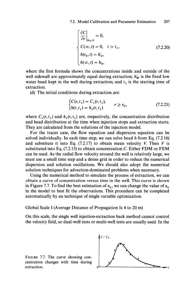
Using the numerical method to simulate the process of extraction, we can
obtain a curve of concentration versus time in the weIl. This curve is shown
in Figure 7.7. To find the best estimation of (XL' we can change the value of (XL
in the model to best fit the observations. This procedure can be completed
automatically by an technique of single variable optimization.
Global Scale I (Average Distance of Propagation Is 4 to 20 m)
On this scale, the single weIl injection-extraction back method cannot control
the velocity field, so dual-weIl tests or multi-weIl tests are usually used. In the
FIGURE 7.7. The curve showing concentration changes with time during
extraction.
CI Co
o~~----------------~~~-
207
OCI = 0
or (ro.t) ,
C(oo,t) =0, t>t1,
(7.2.20)
h(r o , t) = h~,
h( 00, t) = h o ,
where the first formula shows the concentrations inside and outside of the
weIl sidewall are approximately equal during extraction; hiv is the fixed low
water head kept in the weIl during extraction; and t 1 is the starting time of
extraction.
(d) The initial conditions during extraction are:
{
C(r,t d = C1(r,td,
h(r, td = h1 (r, td
(7.2.21)
where Cl (r, t d and h 1 (r, t 1 ) are, respectively, the concentration distribution
and head distribution at the time when injection stops and extraction starts.
They are calculated from the solutions of the injection model.
For the tracer case, the flow equation and dispersion equation can be
solved individuaIly. In each time step, we can solve head h from Eq. (7.2.16)
and substitute it into Eq. (7.2.17) to obtain mean velocity V. Then V is
substituted into Eq. (7.2.15) to obtain concentration C. Either FDM or FEM
can be used. As the radial flow velocity around the weIl is relatively large, we
must use a small time step and a dense grid in order to reduce the numerical
dispersion and solution oscillations. We should also adopt the numerical
solution techniques for advection-dominated problems when necessary.
Using the numerical method to simulate the process of extraction, we can
obtain a curve of concentration versus time in the weIl. This curve is shown
in Figure 7.7. To find the best estimation of (XL' we can change the value of (XL
in the model to best fit the observations. This procedure can be completed
automatically by an technique of single variable optimization.
Global Scale I (Average Distance of Propagation Is 4 to 20 m)
On this scale, the single weIl injection-extraction back method cannot control
the velocity field, so dual-weIl tests or multi-weIl tests are usually used. In the
FIGURE 7.7. The curve showing concentration changes with time during
extraction.
CI Co
o~~----------------~~~-