

6.2. Upstream Weighted Methods
163
be lowered. Some authors ealled it the cross wind phenomenon. In order to
eliminate this phenomenon, Brooks and Hughes (1982) proposed a modified
form named the Streamline Upwind/Petrov-Galerkin (SU/PG) method. In this
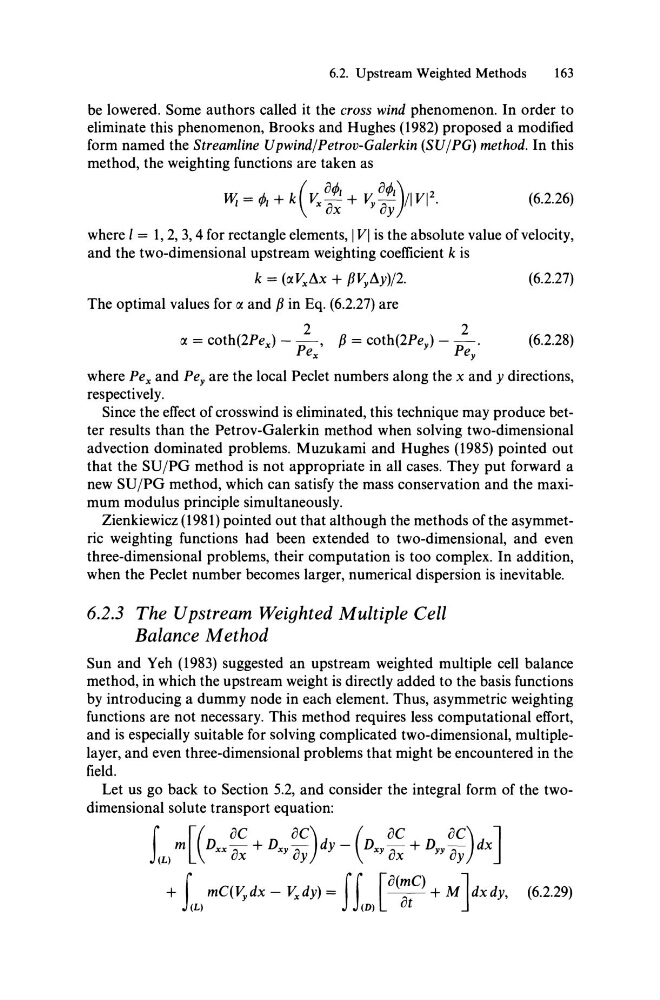
method, the weighting funetions are taken as
( OrPl
OrPl) 2
W, = rPl + k Y" ox + V, oy /IVI .
(6.2.26)
where I = 1, 2, 3,4 for reetangle elements, I VI is the absolute value of velocity,
and the two-dimensional upstream weighting eoeffieient k is
k = (IXVxAx + ßV,Ay)/2.
(6.2.27)
The optimal values for IX and ß in Eq. (6.2.27) are
2
2
IX = eoth(2Pe x ) - - , ß = eoth(2Pey) - -P .
Pex
ey
(6.2.28)
where Pex and Pey are the loeal Peclet numbers along the x and y direetions,
respeetively.
Sinee the effeet of erosswind is eliminated, this teehnique may produce better results than the Petrov-Galerkin method when solving two-dimensional
adveetion dominated problems. Muzukami and Hughes (1985) pointed out
that the SU/PG method is not appropriate in all eases. They put forward a
new SU/PG method, whieh ean satisfy the mass eonservation and the maximum modulus principle simultaneously.
Zienkiewiez (1981) pointed out that although the methods ofthe asymmetrie weighting funetions had been extended to two-dimensional, and even
three-dimensional problems, their eomputation is too eomplex. In addition,
when the Peclet number beeomes larger, numerieal dispersion is inevitable.
6.2.3 The Upstream Weighted Multiple Cell
Balance M ethod
Sun and Yeh (1983) suggested an upstream weighted multiple eell balance
method, in whieh the upstream weight is direetly added to the basis funetions
by introdueing a dummy node in eaeh element. Thus, asymmetrie weighting
funetions are not neeessary. This method requires less eomputational effort,
and is espeeially suitable for solving eomplieated two-dimensional, multiplelayer, and even three-dimensional problems that might be eneountered in the
field.
Let us go baek to Seetion 5.2, and eonsider the integral form of the twodimensional solute transport equation:
i L) m [( Dxx ~~ + D xy ~~) dy - (D xy ~~ + D yy ~~) dX]
+ r mC(V,dx - Y"dy) = f r [a(~C) + M]dXd Y , (6.2.29)
J(L)
J(D)
ut
163
be lowered. Some authors ealled it the cross wind phenomenon. In order to
eliminate this phenomenon, Brooks and Hughes (1982) proposed a modified
form named the Streamline Upwind/Petrov-Galerkin (SU/PG) method. In this
method, the weighting funetions are taken as
( OrPl
OrPl) 2
W, = rPl + k Y" ox + V, oy /IVI .
(6.2.26)
where I = 1, 2, 3,4 for reetangle elements, I VI is the absolute value of velocity,
and the two-dimensional upstream weighting eoeffieient k is
k = (IXVxAx + ßV,Ay)/2.
(6.2.27)
The optimal values for IX and ß in Eq. (6.2.27) are
2
2
IX = eoth(2Pe x ) - - , ß = eoth(2Pey) - -P .
Pex
ey
(6.2.28)
where Pex and Pey are the loeal Peclet numbers along the x and y direetions,
respeetively.
Sinee the effeet of erosswind is eliminated, this teehnique may produce better results than the Petrov-Galerkin method when solving two-dimensional
adveetion dominated problems. Muzukami and Hughes (1985) pointed out
that the SU/PG method is not appropriate in all eases. They put forward a
new SU/PG method, whieh ean satisfy the mass eonservation and the maximum modulus principle simultaneously.
Zienkiewiez (1981) pointed out that although the methods ofthe asymmetrie weighting funetions had been extended to two-dimensional, and even
three-dimensional problems, their eomputation is too eomplex. In addition,
when the Peclet number beeomes larger, numerieal dispersion is inevitable.
6.2.3 The Upstream Weighted Multiple Cell
Balance M ethod
Sun and Yeh (1983) suggested an upstream weighted multiple eell balance
method, in whieh the upstream weight is direetly added to the basis funetions
by introdueing a dummy node in eaeh element. Thus, asymmetrie weighting
funetions are not neeessary. This method requires less eomputational effort,
and is espeeially suitable for solving eomplieated two-dimensional, multiplelayer, and even three-dimensional problems that might be eneountered in the
field.
Let us go baek to Seetion 5.2, and eonsider the integral form of the twodimensional solute transport equation:
i L) m [( Dxx ~~ + D xy ~~) dy - (D xy ~~ + D yy ~~) dX]
+ r mC(V,dx - Y"dy) = f r [a(~C) + M]dXd Y , (6.2.29)
J(L)
J(D)
ut