

5.3. Finite Element Methods for Three-Dimensional Problems
127
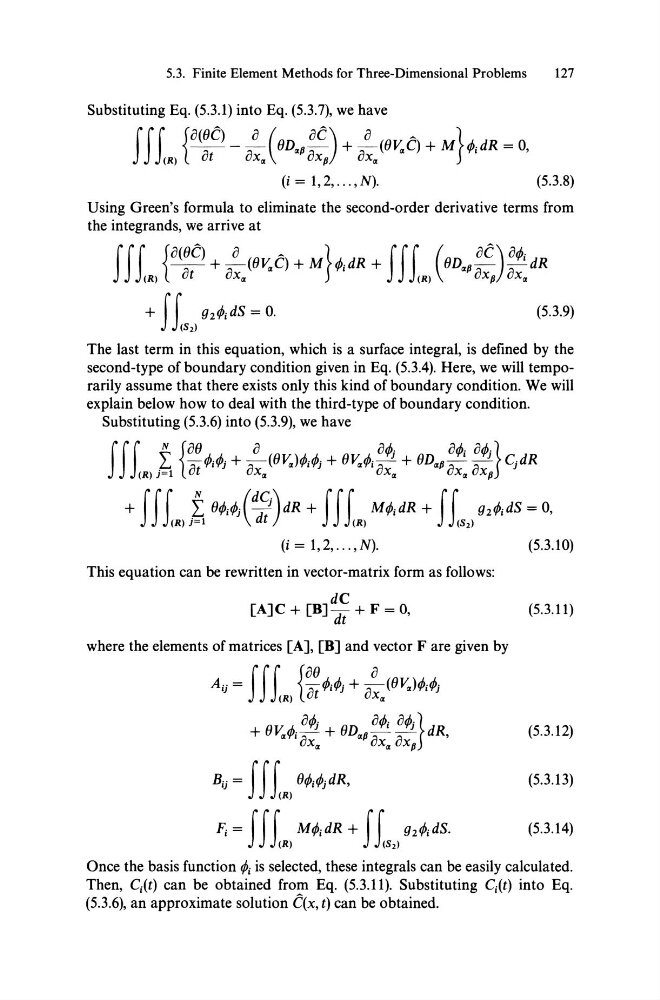
Substituting Eq. (5.3.1) into Eq. (5.3.7), we have
f f IR) {a~;) - a!~ (eD~p :~) + a!~ (e~c) + M} q)i dR = 0,
(i = 1,2, ... , N).
(5.3.8)
Using Green's formula to eliminate the second-order derivative terms from
the integrands, we arrive at
ff r {a(ec) a ~ }
ff r ( ac) aq)i
JR) ----at + ax}e~C) + M q)i dR + JR) eD~p axp ax~ dR
+ f r g2q)i dS = O.
JS2)
(5.3.9)
The last term in this equation, which is a surface integral, is defined by the
second-type of boundary condition given in Eq. (5.3.4). Here, we will temporarily assume that there exists only this kind ofboundary condition. We will
explain below how to deal with the third-type of boundary condition.
Substituting (5.3.6) into (5.3.9), we have
ffi
N {ae
a
aq)j
aq)i aq)j}
~ -a q)iq)j + -a (e~)q)iq)j + e~q)i-a + eD~p-a -a CjdR
(R) J=l
t
x~
x~
x~ xp
+ ff r t eq)iq)j(ddCj)dR + ff r Mq)i dR + fr g2q)i dS = 0,
J (R) J=l
t
J (R)
J (S2)
(i = 1,2, ... , N).
(5.3.10)
This equation can be rewritten in vector-matrix form as follows:
(5.3.11)
where the elements ofmatrices [A], [B] and vector F are given by
Aij = f f IR) g~ q)iq)j + a!~ (e~)q)iq)j
aq)j
aq)i aq)j}
+ e~q)i-a + eD~p-a -a dR,
x~
x~ Xp
(5.3.12)
Bij = f f IR) eq)iq)j dR,
(5.3.13)
Fi = ff r Mq)i dR + fr g2q)i dS.
J(R)
J(S2)
(5.3.14)
Onee the basis function q)i is selected, these integrals can be easily calculated.
Then, Ci(t) can be obtained from Eq. (5.3.11). Substituting Ci(t) into Eq.
(5.3.6), an approximate solution C(x, t) can be obtained.
127
Substituting Eq. (5.3.1) into Eq. (5.3.7), we have
f f IR) {a~;) - a!~ (eD~p :~) + a!~ (e~c) + M} q)i dR = 0,
(i = 1,2, ... , N).
(5.3.8)
Using Green's formula to eliminate the second-order derivative terms from
the integrands, we arrive at
ff r {a(ec) a ~ }
ff r ( ac) aq)i
JR) ----at + ax}e~C) + M q)i dR + JR) eD~p axp ax~ dR
+ f r g2q)i dS = O.
JS2)
(5.3.9)
The last term in this equation, which is a surface integral, is defined by the
second-type of boundary condition given in Eq. (5.3.4). Here, we will temporarily assume that there exists only this kind ofboundary condition. We will
explain below how to deal with the third-type of boundary condition.
Substituting (5.3.6) into (5.3.9), we have
ffi
N {ae
a
aq)j
aq)i aq)j}
~ -a q)iq)j + -a (e~)q)iq)j + e~q)i-a + eD~p-a -a CjdR
(R) J=l
t
x~
x~
x~ xp
+ ff r t eq)iq)j(ddCj)dR + ff r Mq)i dR + fr g2q)i dS = 0,
J (R) J=l
t
J (R)
J (S2)
(i = 1,2, ... , N).
(5.3.10)
This equation can be rewritten in vector-matrix form as follows:
(5.3.11)
where the elements ofmatrices [A], [B] and vector F are given by
Aij = f f IR) g~ q)iq)j + a!~ (e~)q)iq)j
aq)j
aq)i aq)j}
+ e~q)i-a + eD~p-a -a dR,
x~
x~ Xp
(5.3.12)
Bij = f f IR) eq)iq)j dR,
(5.3.13)
Fi = ff r Mq)i dR + fr g2q)i dS.
J(R)
J(S2)
(5.3.14)
Onee the basis function q)i is selected, these integrals can be easily calculated.
Then, Ci(t) can be obtained from Eq. (5.3.11). Substituting Ci(t) into Eq.
(5.3.6), an approximate solution C(x, t) can be obtained.