

128
5. Finite Element Methods for Solving Hydrodynamie Dispersion Equations
If there exists the third-type of boundary condition-Eq. (5.3.5), we must
apply Green's formula to both the dispersion and advection terms of Eq.
(5.3.8) simultaneously. The coefficients of Eq. (5.3.11) then become
(5.3.15a)
(5.3.15b)
(5.3.15c)
It should be noted that the three-dimensional Galerkin FEM is a direct
extension of its two-dimensional form. The principles of selecting basis functions combined with finite element discretization are the same as those in the
two-dimensional case. That is, let rPi be equal to 1 at node i and zero at other
nodes. Such a selection of basis functions will make the coefficient matrices
[A] and [B] of Eq. (5.3.11) turn into highly-sparse matrices. Furthermore,
coefficient Ci(t) in Eq. (5.3.6) is just equal to the concentration of node i at
time t.
The problem left is how to select the shape of elements and the order of
basis functions. The simplest way is by adopting the tetrahedron element and
linear basis functions. As it is inconvenient to input the geometrical information of tetrahedron elements, the combined elements such as triangular prism
and hexahedron are often used. The former can be partitioned into three
tetrahedrons, and the latter into five.
Gupta et al. (1975) used isoparametrie FEM to solve the water quality
equation. Using isoparametric FEM in three-dimensional problems can reduce the number of nodes, and achieve a higher accuracy.
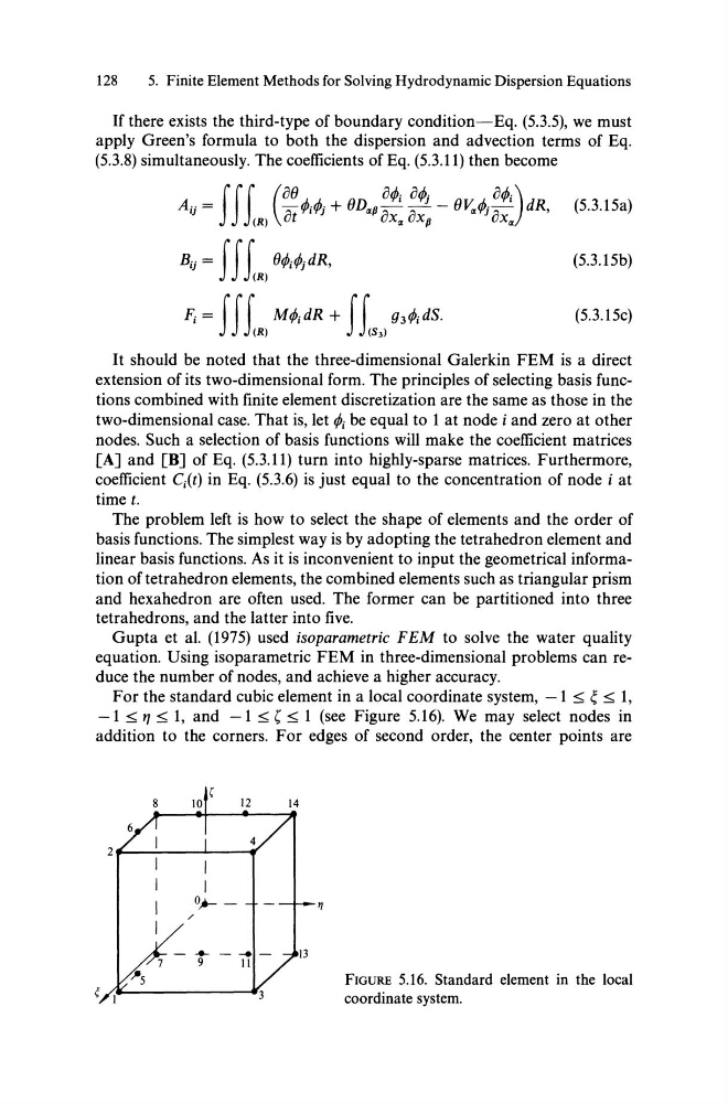
For the standard cubic element in a local coordinate system, -1 :::;; e : : : ; ; 1,
-1 :::;; '1 :::;; 1, and -1:::;;':::;; 1 (see Figure 5.16). We may select nodes in
addition to the corners. For edges of second order, the center points are
,
8
10
12
2F---~--~----~
~ ~I~------------~
14
"
FIGURE 5.16. Standard element in the loeal
eoordinate system.
5. Finite Element Methods for Solving Hydrodynamie Dispersion Equations
If there exists the third-type of boundary condition-Eq. (5.3.5), we must
apply Green's formula to both the dispersion and advection terms of Eq.
(5.3.8) simultaneously. The coefficients of Eq. (5.3.11) then become
(5.3.15a)
(5.3.15b)
(5.3.15c)
It should be noted that the three-dimensional Galerkin FEM is a direct
extension of its two-dimensional form. The principles of selecting basis functions combined with finite element discretization are the same as those in the
two-dimensional case. That is, let rPi be equal to 1 at node i and zero at other
nodes. Such a selection of basis functions will make the coefficient matrices
[A] and [B] of Eq. (5.3.11) turn into highly-sparse matrices. Furthermore,
coefficient Ci(t) in Eq. (5.3.6) is just equal to the concentration of node i at
time t.
The problem left is how to select the shape of elements and the order of
basis functions. The simplest way is by adopting the tetrahedron element and
linear basis functions. As it is inconvenient to input the geometrical information of tetrahedron elements, the combined elements such as triangular prism
and hexahedron are often used. The former can be partitioned into three
tetrahedrons, and the latter into five.
Gupta et al. (1975) used isoparametrie FEM to solve the water quality
equation. Using isoparametric FEM in three-dimensional problems can reduce the number of nodes, and achieve a higher accuracy.
For the standard cubic element in a local coordinate system, -1 :::;; e : : : ; ; 1,
-1 :::;; '1 :::;; 1, and -1:::;;':::;; 1 (see Figure 5.16). We may select nodes in
addition to the corners. For edges of second order, the center points are
,
8
10
12
2F---~--~----~
~ ~I~------------~
14
"
FIGURE 5.16. Standard element in the loeal
eoordinate system.