

126
5. Finite Element Methods for Solving Hydrodynamic Dispersion Equations
sented. Therefore, more and more three-dimensional models were developed
for field problems in recent years.
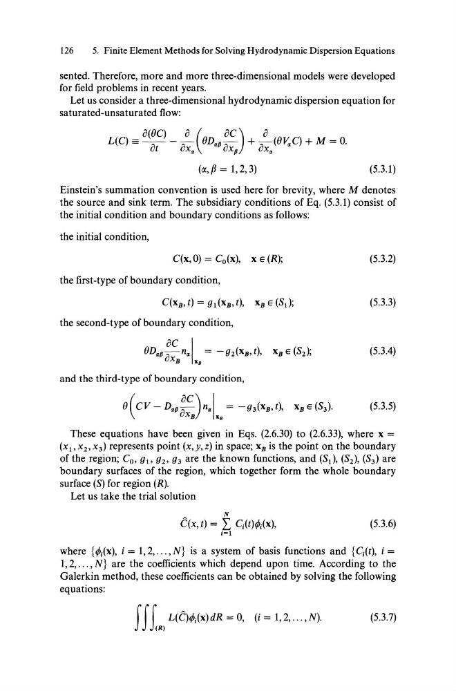
Let us consider a three-dimensional hydrodynamic dispersion equation for
saturated-unsaturated flow:
o(OC)
0 (
OC)
0
L(C) == -~ - - -;- OD ap -;- + -;-(O~C) + M = O.
ut
uX a
uXp
uX a
(rx,ß = 1,2,3)
(5.3.1)
Einstein's summation convention is used here for brevity, where M denotes
the source and sink term. The subsidiary conditions of Eq. (5.3.1) consist of
the initial condition and boundary conditions as folIows:
the initial condition,
C(x,O) = Co (x), x E (R);
(5.3.2)
the first-type of boundary condition,
(5.3.3)
the second-type of boundary condition,
(5.3.4)
and the third-type of boundary condition,
o( CV - D ap :~) naL = -g3(XB, t), XB E (S3).
(5.3.5)
These equations have been given in Eqs. (2.6.30) to (2.6.33), where x =
(Xl' X 2 , X 3 ) represents point (x,y, z) in space; XB is the point on the boundary
of the region; Co, gl, g2, g3 are the known functions, and (Sl)' (S2), (S3) are
boundary surfaces of the region, which together form the whole boundary
surface (S) for region (R).
Let us take the trial solution
N
C(x, t) = L Ci(t)tMx),
(5.3.6)
i=l
where {tMx), i = 1,2, ... , N} is a system of basis functions and {Ci(t), i =
1,2, ... , N} are the coefficients which depend upon time. According to the
Galerkin method, these coefficients can be obtained by solving the following
equations:
f f IR) L(c)(Mx)dR = 0, (i = 1,2, ... ,N).
(5.3.7)
5. Finite Element Methods for Solving Hydrodynamic Dispersion Equations
sented. Therefore, more and more three-dimensional models were developed
for field problems in recent years.
Let us consider a three-dimensional hydrodynamic dispersion equation for
saturated-unsaturated flow:
o(OC)
0 (
OC)
0
L(C) == -~ - - -;- OD ap -;- + -;-(O~C) + M = O.
ut
uX a
uXp
uX a
(rx,ß = 1,2,3)
(5.3.1)
Einstein's summation convention is used here for brevity, where M denotes
the source and sink term. The subsidiary conditions of Eq. (5.3.1) consist of
the initial condition and boundary conditions as folIows:
the initial condition,
C(x,O) = Co (x), x E (R);
(5.3.2)
the first-type of boundary condition,
(5.3.3)
the second-type of boundary condition,
(5.3.4)
and the third-type of boundary condition,
o( CV - D ap :~) naL = -g3(XB, t), XB E (S3).
(5.3.5)
These equations have been given in Eqs. (2.6.30) to (2.6.33), where x =
(Xl' X 2 , X 3 ) represents point (x,y, z) in space; XB is the point on the boundary
of the region; Co, gl, g2, g3 are the known functions, and (Sl)' (S2), (S3) are
boundary surfaces of the region, which together form the whole boundary
surface (S) for region (R).
Let us take the trial solution
N
C(x, t) = L Ci(t)tMx),
(5.3.6)
i=l
where {tMx), i = 1,2, ... , N} is a system of basis functions and {Ci(t), i =
1,2, ... , N} are the coefficients which depend upon time. According to the
Galerkin method, these coefficients can be obtained by solving the following
equations:
f f IR) L(c)(Mx)dR = 0, (i = 1,2, ... ,N).
(5.3.7)