

5.3. Finite Element Methods for Three-Dimensional Problems
125
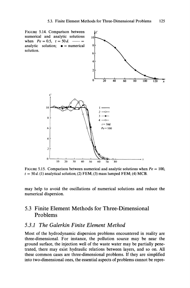
FIGURE 5.14. Comparison between
c
numerical and analytic solutions
when Pe = 0.5, t = 50d. - - =
analytic solution; • = numerical
solution.
c
8
6
4
2
1 - -
2-03 -
4 ---01= 50d
Pe= 100
o '---::---::-':--L---:'-_-'--~-=~-G:"-_ _ _ _ _ x
10
20
30
40
50
60
70
80
x
FIGURE 5.15. Comparison between numerical and analytic solutions when Pe = 100,
t = 50d. (1) analytical solution; (2) FEM; (3) mass lumped FEM; (4) MCB.
may help to avoid the oscillations of numerical solutions and reduce the
numerical dispersion.
5.3 Finite Element Methods for Three-Dimensional
Problems
5.3.1 The Galerkin Finite Element Method
Most of the hydrodynamic dispersion problems encountered in reality are
three-dimensional. For instance, the pollution source may be near the
ground surface, the injection well of the waste water may be partially penetrated, there may exist hydraulic relations between layers, and so on. All
these common cases are three-dimensional problems. If they are simplified
into two-dimensional ones, the essential aspects of problems cannot be repre-
125
FIGURE 5.14. Comparison between
c
numerical and analytic solutions
when Pe = 0.5, t = 50d. - - =
analytic solution; • = numerical
solution.
c
8
6
4
2
1 - -
2-03 -
4 ---01= 50d
Pe= 100
o '---::---::-':--L---:'-_-'--~-=~-G:"-_ _ _ _ _ x
10
20
30
40
50
60
70
80
x
FIGURE 5.15. Comparison between numerical and analytic solutions when Pe = 100,
t = 50d. (1) analytical solution; (2) FEM; (3) mass lumped FEM; (4) MCB.
may help to avoid the oscillations of numerical solutions and reduce the
numerical dispersion.
5.3 Finite Element Methods for Three-Dimensional
Problems
5.3.1 The Galerkin Finite Element Method
Most of the hydrodynamic dispersion problems encountered in reality are
three-dimensional. For instance, the pollution source may be near the
ground surface, the injection well of the waste water may be partially penetrated, there may exist hydraulic relations between layers, and so on. All
these common cases are three-dimensional problems. If they are simplified
into two-dimensional ones, the essential aspects of problems cannot be repre-