

124
5. Finite Element Methods for Solving Hydrodynamic Dispersion Equations
,~==m·
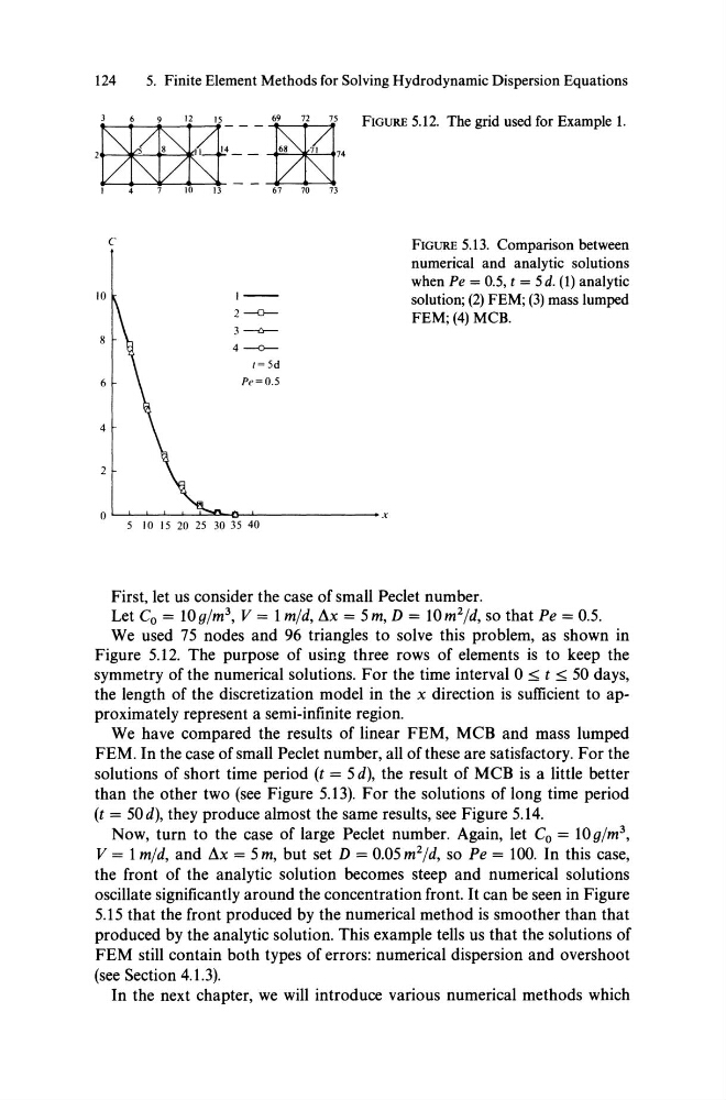
FIGURE 5.12. The grid used for Example 1.
I
4
7
10
13
67
70
73
10
8
6
4
2
0
C
1 - -
2-0-3 ---6-4 - 0 -
1=5d
Pe=0.5
5 10 15 20 25 3035 40
x
FIGURE 5.13. Comparison between
numerical and analytic solutions
when Pe = 0.5, t = 5 d. (1) analytic
solution; (2) FEM; (3) mass lumped
FEM; (4) MCB.
First, let us consider the case of small Peclet number.
Let Co = lOg/m 3 , V = 1 m/d, ßx = 5 m, D = 10m 2 /d, so that Pe = 0.5.
We used 75 nodes and 96 triangles to solve this problem, as shown in
Figure 5.12. The purpose of using three rows of elements is to keep the
symmetry of the numerical solutions. For the time interval 0 ::s;; t::s;; 50 days,
the length of the discretization model in the x direction is sufficient to approximately represent a semi-infinite region.
We have compared the results of linear FEM, MCB and mass lumped
FEM. In the case of small Pec1et number, all of these are satisfactory. For the
solutions of short time period (t = 5 d), the result of MCB is a little better
than the other two (see Figure 5.13). For the solutions of long time period
(t = 50d), they produce almost the same results, see Figure 5.14.
Now, turn to the case of large Pec1et number. Again, let Co = 10g/ml,
V = 1 m/d, and ßx = 5 m, but set D = 0.05 m 2 /d, so Pe = 100. In this case,
the front of the analytic solution becomes steep and numerical solutions
oscillate significantly around the concentration front. It can be seen in Figure
5.15 that the front produced by the numerical method is smoother than that
produced by the analytic solution. This example teIls us that the solutions of
FEM still contain both types of errors: numerical dispersion and overshoot
(see Section 4.1.3).
In the next chapter, we will introduce various numerical methods which
5. Finite Element Methods for Solving Hydrodynamic Dispersion Equations
,~==m·
FIGURE 5.12. The grid used for Example 1.
I
4
7
10
13
67
70
73
10
8
6
4
2
0
C
1 - -
2-0-3 ---6-4 - 0 -
1=5d
Pe=0.5
5 10 15 20 25 3035 40
x
FIGURE 5.13. Comparison between
numerical and analytic solutions
when Pe = 0.5, t = 5 d. (1) analytic
solution; (2) FEM; (3) mass lumped
FEM; (4) MCB.
First, let us consider the case of small Peclet number.
Let Co = lOg/m 3 , V = 1 m/d, ßx = 5 m, D = 10m 2 /d, so that Pe = 0.5.
We used 75 nodes and 96 triangles to solve this problem, as shown in
Figure 5.12. The purpose of using three rows of elements is to keep the
symmetry of the numerical solutions. For the time interval 0 ::s;; t::s;; 50 days,
the length of the discretization model in the x direction is sufficient to approximately represent a semi-infinite region.
We have compared the results of linear FEM, MCB and mass lumped
FEM. In the case of small Pec1et number, all of these are satisfactory. For the
solutions of short time period (t = 5 d), the result of MCB is a little better
than the other two (see Figure 5.13). For the solutions of long time period
(t = 50d), they produce almost the same results, see Figure 5.14.
Now, turn to the case of large Pec1et number. Again, let Co = 10g/ml,
V = 1 m/d, and ßx = 5 m, but set D = 0.05 m 2 /d, so Pe = 100. In this case,
the front of the analytic solution becomes steep and numerical solutions
oscillate significantly around the concentration front. It can be seen in Figure
5.15 that the front produced by the numerical method is smoother than that
produced by the analytic solution. This example teIls us that the solutions of
FEM still contain both types of errors: numerical dispersion and overshoot
(see Section 4.1.3).
In the next chapter, we will introduce various numerical methods which