

5.2. The Multiple Cell Balance Method
123
Therefore, a program written for the multiple cell balance method can be
turned into a pro gram for Galerkin's FEM by changing only two constants.
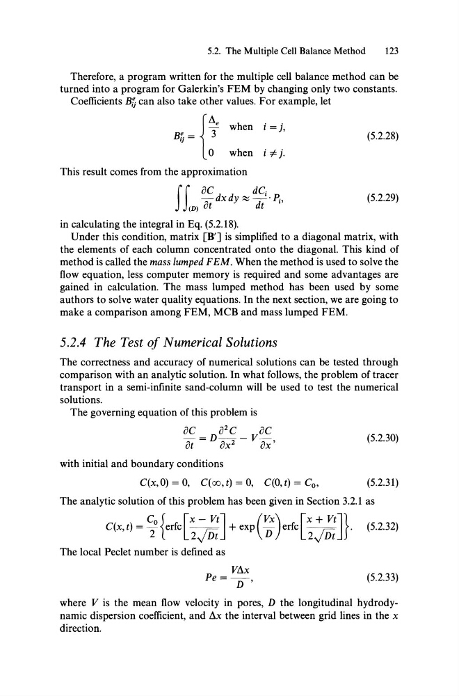
Coefficients Bij can also take other values. For example, let
e _ {~e when i = j,
Bijo when i #j.
(5.2.28)
This result comes from the approximation
ff
oC
dCi
TdxdY~-d . Pi'
CD) ut
t
(5.2.29)
in calculating the integral in Eq. (5.2.18).
Under this condition, matrix [B'] is simplified to a diagonal matrix, with
the elements of each column concentrated onto the diagonal. This kind of
method is called the mass lumped FEM. When the method is used to solve the
flow equation, less computer memory is required and some advantages are
gained in calculation. The mass lumped method has been used by some
authors to solve water quality equations. In the next section, we are going to
make a comparison among FEM, MCB and mass lumped FEM.
5.2.4 The Test of Numerical Solutions
The correctness and accuracy of numerical solutions can be tested through
comparison with an analytic solution. In what follows, the problem of tracer
transport in a semi-infinite sand-column will be used to test the numerical
solutions.
The governing equation of this problem is
OC = D o2C _ voC
ot
ox 2
ox'
(5.2.30)
with initial and boundary conditions
C(x,O) = 0, C( 00, t) = 0, C(O, t) = Co,
(5.2.31)
The analytic solution ofthis problem has been given in Section 3.2.1 as
C(x,t) = ~O{erfc[~~J + exp(~)erfc[~~J}. (5.2.32)
The local Pec1et number is defined as
Pe = VAx
D'
(5.2.33)
where V is the mean flow velocity in pores, D the longitudinal hydrodynamic dispersion coefficient, and Ax the interval between grid lines in the x
direction.
123
Therefore, a program written for the multiple cell balance method can be
turned into a pro gram for Galerkin's FEM by changing only two constants.
Coefficients Bij can also take other values. For example, let
e _ {~e when i = j,
Bijo when i #j.
(5.2.28)
This result comes from the approximation
ff
oC
dCi
TdxdY~-d . Pi'
CD) ut
t
(5.2.29)
in calculating the integral in Eq. (5.2.18).
Under this condition, matrix [B'] is simplified to a diagonal matrix, with
the elements of each column concentrated onto the diagonal. This kind of
method is called the mass lumped FEM. When the method is used to solve the
flow equation, less computer memory is required and some advantages are
gained in calculation. The mass lumped method has been used by some
authors to solve water quality equations. In the next section, we are going to
make a comparison among FEM, MCB and mass lumped FEM.
5.2.4 The Test of Numerical Solutions
The correctness and accuracy of numerical solutions can be tested through
comparison with an analytic solution. In what follows, the problem of tracer
transport in a semi-infinite sand-column will be used to test the numerical
solutions.
The governing equation of this problem is
OC = D o2C _ voC
ot
ox 2
ox'
(5.2.30)
with initial and boundary conditions
C(x,O) = 0, C( 00, t) = 0, C(O, t) = Co,
(5.2.31)
The analytic solution ofthis problem has been given in Section 3.2.1 as
C(x,t) = ~O{erfc[~~J + exp(~)erfc[~~J}. (5.2.32)
The local Pec1et number is defined as
Pe = VAx
D'
(5.2.33)
where V is the mean flow velocity in pores, D the longitudinal hydrodynamic dispersion coefficient, and Ax the interval between grid lines in the x
direction.