

122
5. Finite Element Methods for Solving Hydrodynamic Dispersion Equations
A FORTAN program of the MCB is given in Appendix B, in which all
steps of the method are explained in detail.
5.2.3 Comparing with the Finite Element Method
It is interesting to make a comparison between Eqs. (5.2.25) and the discrete
equations obtained from the linear Galerkin FEM.
Letting thickness m = constant and div V = 0, Eq. (5.2.1) then reduces to
Eq. (5.1.1), where 1= -(C'W)/(nm). The coefficients Clfl of Eq. (5.2.10) are
reduced to
1
Clfl = - 4~ [D~xbib, + D~y(Cib, + bic,) + D;yCiC,].
e
Furthermore, let velocity components V': and v,e, be constant in each element. Coefficients ßij in Eq. (5.2.13) are then simplified to
1
ßij = 6(v':b, + v,ec,).
Since div V = 0, all YiI in Eq. (5.2.14) are equal to zero. From am/at = 0, all (jij
in Eq. (5.2.19) are also equal to zero. Therefore, coefficients Ai" given by Eq.
(5.2.22), are simplified to
Ai, = 4~ [D~xbib, + D~y(biC, + Ci b,) + D;ycic,]
e
+ ~(v':b, + v,ec,).
(5.2.26)
Comparing this formula with Eq. (5.1.35), we find that matrix [A'] is exactly
the same as matrix [A] obtained by the Galerkin FEM using linear triangle
elements.
Now let us study the relationship of coefficient matrices [B'] and [B].
When m = constant, Bi) in Eq. (5.2.18) becomes
I
~e 22
. .
3' 36 when I =J,
Bi) = l~ 7
(5.2.27)
3 e • 36 when i =F j.
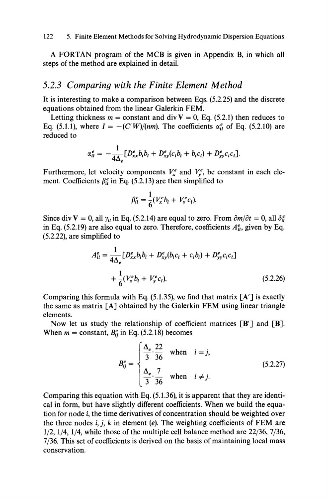
Comparing this equation with Eq. (5.1.36), it is apparent that they are identical in form, but have slightly different coefficients. When we build the equation for node i, the time derivatives of concentration should be weighted over
the three nodes i, j, k in element (e). The weighting coefficients of FEM are
1/2, 1/4, 1/4, while those of the multiple cell balance method are 22/36, 7/36,
7/36. This set of coefficients is derived on the basis of maintaining local mass
conservation.
5. Finite Element Methods for Solving Hydrodynamic Dispersion Equations
A FORTAN program of the MCB is given in Appendix B, in which all
steps of the method are explained in detail.
5.2.3 Comparing with the Finite Element Method
It is interesting to make a comparison between Eqs. (5.2.25) and the discrete
equations obtained from the linear Galerkin FEM.
Letting thickness m = constant and div V = 0, Eq. (5.2.1) then reduces to
Eq. (5.1.1), where 1= -(C'W)/(nm). The coefficients Clfl of Eq. (5.2.10) are
reduced to
1
Clfl = - 4~ [D~xbib, + D~y(Cib, + bic,) + D;yCiC,].
e
Furthermore, let velocity components V': and v,e, be constant in each element. Coefficients ßij in Eq. (5.2.13) are then simplified to
1
ßij = 6(v':b, + v,ec,).
Since div V = 0, all YiI in Eq. (5.2.14) are equal to zero. From am/at = 0, all (jij
in Eq. (5.2.19) are also equal to zero. Therefore, coefficients Ai" given by Eq.
(5.2.22), are simplified to
Ai, = 4~ [D~xbib, + D~y(biC, + Ci b,) + D;ycic,]
e
+ ~(v':b, + v,ec,).
(5.2.26)
Comparing this formula with Eq. (5.1.35), we find that matrix [A'] is exactly
the same as matrix [A] obtained by the Galerkin FEM using linear triangle
elements.
Now let us study the relationship of coefficient matrices [B'] and [B].
When m = constant, Bi) in Eq. (5.2.18) becomes
I
~e 22
. .
3' 36 when I =J,
Bi) = l~ 7
(5.2.27)
3 e • 36 when i =F j.
Comparing this equation with Eq. (5.1.36), it is apparent that they are identical in form, but have slightly different coefficients. When we build the equation for node i, the time derivatives of concentration should be weighted over
the three nodes i, j, k in element (e). The weighting coefficients of FEM are
1/2, 1/4, 1/4, while those of the multiple cell balance method are 22/36, 7/36,
7/36. This set of coefficients is derived on the basis of maintaining local mass
conservation.