

5.2. The Multiple Cell Balance Method
121
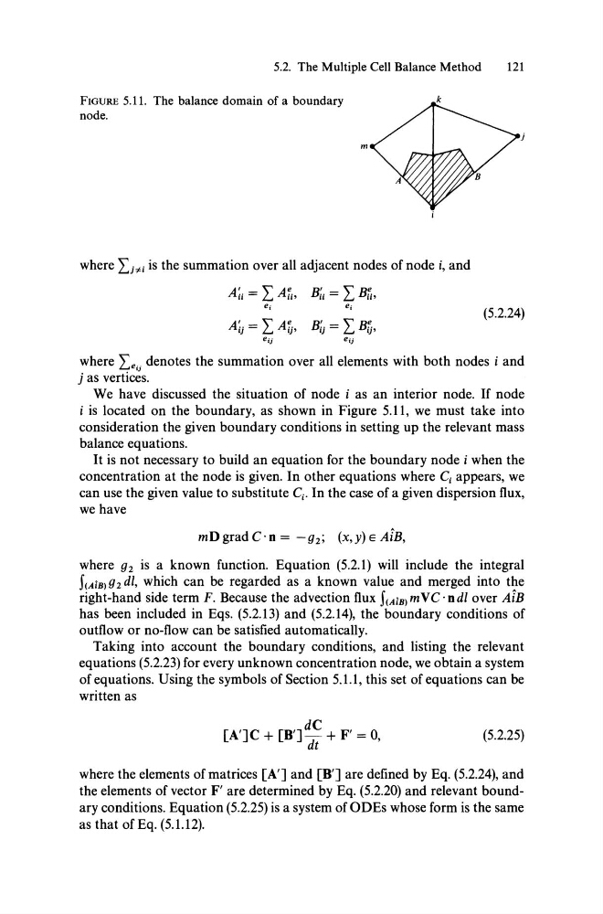
FIGURE 5.11. The balance domain of a boundary
node.
m
k
where Li,<; is the summation over all adjacent nodes of node i, and
A;i = LAii, B;i = LBü,
e.
e.
(5.2.24)
where Leij denotes the summation over all elements with both nodes i and
j as vertices.
We have discussed the situation of node i as an interior node. If node
i is located on the boundary, as shown in Figure 5.11, we must take into
consideration the given boundary conditions in setting up the relevant mass
balance equations.
It is not necessary to build an equation for the boundary node i when the
concentration at the node is given. In other equations where Ci appears, we
can use the given value to substitute Ci. In the case of a given dispersion flux,
we have
mDgradC·o= -92; (x,y)eAiB,
where 92 is a known function. Equation (5.2.1) will include the integral
f(A1B)92d1, which can be regarded as a known value and merged into the
right-hand side term F. Because the advection flux f(A1B) mV C . 0 dl over AiB
has been included in Eqs. (5.2.13) and (5.2.14), the boundary conditions of
outflow or no-flow can be satisfied automatically.
Taking into account the boundary conditions, and listing the relevant
equations (5.2.23) for every unknown concentration node, we obtain a system
of equations. Using the symbols of Section 5.1.1, this set of equations can be
written as
[A']C + [B'] dd~ + F' = 0,
(5.2.25)
where the elements of matrices [A'] and [B'] are defined by Eq. (5.2.24), and
the elements of vector F' are determined by Eq. (5.2.20) and relevant boundary conditions. Equation (5.2.25) is a system ofODEs whose form is the same
as that of Eq. (5.1.12).
121
FIGURE 5.11. The balance domain of a boundary
node.
m
k
where Li,<; is the summation over all adjacent nodes of node i, and
A;i = LAii, B;i = LBü,
e.
e.
(5.2.24)
where Leij denotes the summation over all elements with both nodes i and
j as vertices.
We have discussed the situation of node i as an interior node. If node
i is located on the boundary, as shown in Figure 5.11, we must take into
consideration the given boundary conditions in setting up the relevant mass
balance equations.
It is not necessary to build an equation for the boundary node i when the
concentration at the node is given. In other equations where Ci appears, we
can use the given value to substitute Ci. In the case of a given dispersion flux,
we have
mDgradC·o= -92; (x,y)eAiB,
where 92 is a known function. Equation (5.2.1) will include the integral
f(A1B)92d1, which can be regarded as a known value and merged into the
right-hand side term F. Because the advection flux f(A1B) mV C . 0 dl over AiB
has been included in Eqs. (5.2.13) and (5.2.14), the boundary conditions of
outflow or no-flow can be satisfied automatically.
Taking into account the boundary conditions, and listing the relevant
equations (5.2.23) for every unknown concentration node, we obtain a system
of equations. Using the symbols of Section 5.1.1, this set of equations can be
written as
[A']C + [B'] dd~ + F' = 0,
(5.2.25)
where the elements of matrices [A'] and [B'] are defined by Eq. (5.2.24), and
the elements of vector F' are determined by Eq. (5.2.20) and relevant boundary conditions. Equation (5.2.25) is a system ofODEs whose form is the same
as that of Eq. (5.1.12).