

102
5. Finite Element Methods for Solving Hydrodynamic Dispersion Equations
(5.1.29)
(5.1.30)
where (r 2 ,m) is the common boundary of (R m ) and (r2).
Let the ith basis function (Mx, y) be associated with the ith node and let
{
I whenj = i,
(Mxj'Y) = ~ij = 0 whenj"# i,
(5.1.31)
where (Xj' Yj) are the coordinates of node j. Equation (5.1.31) means that the
value of (Mx, y) is defined to be 1 at node i, and zero at other nodes. Furthermore, we define (Mx, y) as non-zero only in those elements which link up with
node i, and to be always zero in other elements.
These two stipulations have several advantages. First, because A ij and Bij
given in Eqs. (5.1.28) and (5.1.29) are non-zero only when nodes i and j are
in the same element, coefficient matrices [A] and [B] now become highly
sparse. Second, we do not need to integrate on the whole domain (R) for
calculating Aij and Bij. To calculate them we only need to integrate on the
elements that have common nodes i and j. Third, from the definition of Eq.
(5.1.31), the solutions C,+41 of Eq. (5.1.12) are just the unknown nodal values
of approximate solution C at the time t + M, so we do not need go back
to Eq. (5.1.5). Therefore, when we combine the finite element discretization
with the Galerkin method, the calculation process demonstrated in Section
5.1.1 will be much simplified. It is quite evident that even though the above
stipulations are satisfied, the shape of elements, the arrangement of nodes
and the expressions of basis functions are still undetermined. In other words,
we still have a great deal of flexibility in selecting a Galerkin finite element
method.
Two commonly-used options for solving advection-dispersion equations
are given below.
Triangular Elements and Linear Basis Functions
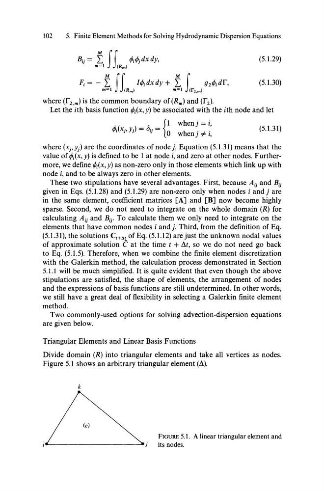
Divide domain (R) into triangular elements and take all vertices as nodes.
Figure 5.1 shows an arbitrary triangular element (A).
k
FIGURE 5.1. A linear triangular element and
_-----------"j
its nodes.
5. Finite Element Methods for Solving Hydrodynamic Dispersion Equations
(5.1.29)
(5.1.30)
where (r 2 ,m) is the common boundary of (R m ) and (r2).
Let the ith basis function (Mx, y) be associated with the ith node and let
{
I whenj = i,
(Mxj'Y) = ~ij = 0 whenj"# i,
(5.1.31)
where (Xj' Yj) are the coordinates of node j. Equation (5.1.31) means that the
value of (Mx, y) is defined to be 1 at node i, and zero at other nodes. Furthermore, we define (Mx, y) as non-zero only in those elements which link up with
node i, and to be always zero in other elements.
These two stipulations have several advantages. First, because A ij and Bij
given in Eqs. (5.1.28) and (5.1.29) are non-zero only when nodes i and j are
in the same element, coefficient matrices [A] and [B] now become highly
sparse. Second, we do not need to integrate on the whole domain (R) for
calculating Aij and Bij. To calculate them we only need to integrate on the
elements that have common nodes i and j. Third, from the definition of Eq.
(5.1.31), the solutions C,+41 of Eq. (5.1.12) are just the unknown nodal values
of approximate solution C at the time t + M, so we do not need go back
to Eq. (5.1.5). Therefore, when we combine the finite element discretization
with the Galerkin method, the calculation process demonstrated in Section
5.1.1 will be much simplified. It is quite evident that even though the above
stipulations are satisfied, the shape of elements, the arrangement of nodes
and the expressions of basis functions are still undetermined. In other words,
we still have a great deal of flexibility in selecting a Galerkin finite element
method.
Two commonly-used options for solving advection-dispersion equations
are given below.
Triangular Elements and Linear Basis Functions
Divide domain (R) into triangular elements and take all vertices as nodes.
Figure 5.1 shows an arbitrary triangular element (A).
k
FIGURE 5.1. A linear triangular element and
_-----------"j
its nodes.