

5.1. Finite Element Methods for Two-Dimensional Problems
101
Collocation Method
In this method, N points (Xi' Yi), i = 1, 2, .. , N, are selected from the domain
(R) and called collocation points. The weighting functions are then defined as
W;(X, y) = !5(x - x;)· !5(y - y;)
(i = 1,2, ... ,N)
(5.1.23)
where !5(x - x;) and c5(y - Yi) are Dirac-c5 functions. H implies that the value
of W;(x, y) is non-zero only at the collocation point (Xi> Yi), and also, for any
function a(x, Y), we have
f r a(x, y) W;(x, y) dx dy = a(x i , y;).
JR)
(5.1.24)
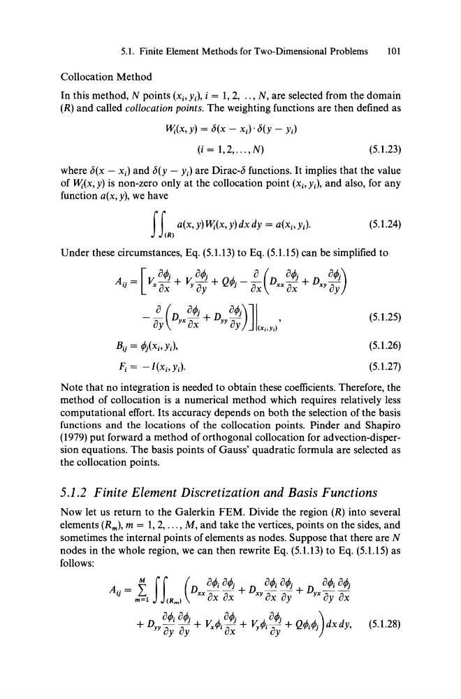
Under these circumstances, Eq. (5.1.13) to Eq. (5.1.15) can be simplified to
[ or!J.
or!J.
0 (0r!J.
or!J.)
Aij = ~ 0: + v, 0; + Qr!Jj - OX Dxx 0: + Dxy 0;
Bij = r!Jj(xi, Yi)'
Fi = -I(xi'Y;).
(5.1.25)
(5.1.26)
(5.1.27)
Note that no integration is needed to obtain these coefficients. Therefore, the
method of collocation is a numerical method which requires relatively less
computational effort. Hs accuracy depends on both the selection of the basis
functions and the locations of the collocation points. Pinder and Shapiro
(1979) put forward a method of orthogonal collocation for advection-dispersion equations. The basis points of Gauss' quadratic formula are selected as
the collocation points.
5.1.2 Finite Element Discretization and Basis Functions
Now let us return to the Galerkin FEM. Divide the region (R) into several
elements (R m ), m = 1,2, ... , M, and take the vertices, points on the sides, and
sometimes the internal points of elements as nodes. Suppose that there are N
nodes in the whole region, we can then rewrite Eq. (5.1.13) to Eq. (5.1.15) as
follows:
(5.1.28)
101
Collocation Method
In this method, N points (Xi' Yi), i = 1, 2, .. , N, are selected from the domain
(R) and called collocation points. The weighting functions are then defined as
W;(X, y) = !5(x - x;)· !5(y - y;)
(i = 1,2, ... ,N)
(5.1.23)
where !5(x - x;) and c5(y - Yi) are Dirac-c5 functions. H implies that the value
of W;(x, y) is non-zero only at the collocation point (Xi> Yi), and also, for any
function a(x, Y), we have
f r a(x, y) W;(x, y) dx dy = a(x i , y;).
JR)
(5.1.24)
Under these circumstances, Eq. (5.1.13) to Eq. (5.1.15) can be simplified to
[ or!J.
or!J.
0 (0r!J.
or!J.)
Aij = ~ 0: + v, 0; + Qr!Jj - OX Dxx 0: + Dxy 0;
Bij = r!Jj(xi, Yi)'
Fi = -I(xi'Y;).
(5.1.25)
(5.1.26)
(5.1.27)
Note that no integration is needed to obtain these coefficients. Therefore, the
method of collocation is a numerical method which requires relatively less
computational effort. Hs accuracy depends on both the selection of the basis
functions and the locations of the collocation points. Pinder and Shapiro
(1979) put forward a method of orthogonal collocation for advection-dispersion equations. The basis points of Gauss' quadratic formula are selected as
the collocation points.
5.1.2 Finite Element Discretization and Basis Functions
Now let us return to the Galerkin FEM. Divide the region (R) into several
elements (R m ), m = 1,2, ... , M, and take the vertices, points on the sides, and
sometimes the internal points of elements as nodes. Suppose that there are N
nodes in the whole region, we can then rewrite Eq. (5.1.13) to Eq. (5.1.15) as
follows:
(5.1.28)