

100
5. Finite Element Methods for Solving Hydrodynamic Dispersion Equations
Equation (5.1.17) is a system oflinear algebraie equations. It ean be solved by
either the iteration method or the direet method. At the end of this ehapter
we will diseuss these methods. Note that beeause of the existence of adveetion
terms in the adveetion-dispersion equation, eoeffieient matrix [A] is not
symmetrie. This faet ean be clearly seen from the strueture of Eq. (5.1.13).
Therefore, [E] in Eq. (5.1.17) is not a symmetrie matrix either. This is the
major difTerence between the finite element equations for mass transport
problems and for groundwater flow problems. When [E] is an asymmetrie
matrix, the direet solution method requires more storage spaee and eomputational efTort.
After solving Ct + 4t from Eq. (5.1.17), the approximate solution C at t + Ilt
ean be obtained by substituting C t + 4t into the right-hand side of Eq. (5.1.5).
These are the main steps of solving adveetion-dispersion equations with
the method of weighted residuals. The remaining problem is how to ehoose
the basis and weighting funetions for simplifying the ealeulation of the eoeffieient matriees.
Galerkin Method
The Galerkin method uses the basis funetions in Eq. (5.1.6) as the weighting
funetions. We shall explain this method in detail in the following seetions.
Subdomain Method
The method of subdomain is also ealled the method of element collocation.
Subdivide the region (R) into several elements, and denote as (R;), i = 1, 2,
... , N. Let each element be assoeiated with a weighting funetion, and define
the weighting funetions as:
( ) {
I when (x,y) E (R j ),
Wx,y =
,
0 when (x, y) ~ (R j ).
(5.1.19)
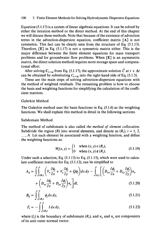
Under sueh a seleetion, Eq. (5.1.13) to Eq. (5.1.15), whieh were used to calculate eoefficient matriees for Eq. (5.1.12), ean be simplified to
(5.1.20)
(5.1.21)
(5.1.22)
where (li) is the boundary of subdomain (R j ), and n x and ny are eomponents
of its unit outer normal vector.
5. Finite Element Methods for Solving Hydrodynamic Dispersion Equations
Equation (5.1.17) is a system oflinear algebraie equations. It ean be solved by
either the iteration method or the direet method. At the end of this ehapter
we will diseuss these methods. Note that beeause of the existence of adveetion
terms in the adveetion-dispersion equation, eoeffieient matrix [A] is not
symmetrie. This faet ean be clearly seen from the strueture of Eq. (5.1.13).
Therefore, [E] in Eq. (5.1.17) is not a symmetrie matrix either. This is the
major difTerence between the finite element equations for mass transport
problems and for groundwater flow problems. When [E] is an asymmetrie
matrix, the direet solution method requires more storage spaee and eomputational efTort.
After solving Ct + 4t from Eq. (5.1.17), the approximate solution C at t + Ilt
ean be obtained by substituting C t + 4t into the right-hand side of Eq. (5.1.5).
These are the main steps of solving adveetion-dispersion equations with
the method of weighted residuals. The remaining problem is how to ehoose
the basis and weighting funetions for simplifying the ealeulation of the eoeffieient matriees.
Galerkin Method
The Galerkin method uses the basis funetions in Eq. (5.1.6) as the weighting
funetions. We shall explain this method in detail in the following seetions.
Subdomain Method
The method of subdomain is also ealled the method of element collocation.
Subdivide the region (R) into several elements, and denote as (R;), i = 1, 2,
... , N. Let each element be assoeiated with a weighting funetion, and define
the weighting funetions as:
( ) {
I when (x,y) E (R j ),
Wx,y =
,
0 when (x, y) ~ (R j ).
(5.1.19)
Under sueh a seleetion, Eq. (5.1.13) to Eq. (5.1.15), whieh were used to calculate eoefficient matriees for Eq. (5.1.12), ean be simplified to
(5.1.20)
(5.1.21)
(5.1.22)
where (li) is the boundary of subdomain (R j ), and n x and ny are eomponents
of its unit outer normal vector.