

5.1. Finite Element Methods for Two-Dimensional Problems
99
The last term on the left-hand side ofthe above equation is obtained from the
second-type boundary condition in Eq. (5.1.4).
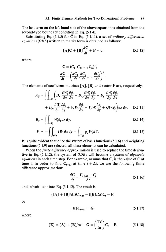
Substituting Eq. (5.1.5) for ein Eq. (5.1.11), a set of ordinary differential
equations (ODE) written in matrix form is obtained as follows:
where
dC
[A]C + [B]Tt + F = 0,
C = (Cl ,C2 , ••• ,CNf,
dC _ (dCl dC2
dCN)T
Tt - (ft'(ft' ... '(ft .
(5.1.12)
The elements of coefficient matrices [A], [B] and vector F are, respectively:
f r ( oW o,p. oW o,p. oW o,p.
Aij = J(Rl D xx ox' o~ + D xy ox' 0; + D yx Oy' o~
aw a,p.
o,p.
a,p.
)
+ Dyy Oy' 0; + YxWia~ + V,Wi a ; + QWi,pj dxdy, (5.1.13)
Rij = f r Wi,pj dx dy,
JRl
Fi = -f r lWidxdy + r g2 Widr.
J(Rl
J(r2l
(5.1.14)
(5.1.15)
It is quite evident that once the system ofbasis functions (5.1.6) and weighting
functions (5.1.9) are selected, all these elements can be calculated.
When the finite diJJerence approximation is used to replace the time derivative in Eq. (5.1.12), the system of ODEs will become a system of algebraic
equations in each time step. For example, assume that C t is the value of C at
time t. In order to find CtHt at time t + At, we use the following finite
difference approximation:
dC C tHt - C t
Tt- At
(5.1.16)
and substitute it into Eq. (5.1.12). The result is
([A] + [B]/At)CtHt = ([B]/L\t)Ct - F,
or
[E] C tHt = G,
(5.1.17)
where
[E] = [A] + [B]/L\t; G = ([:;)C t - F.
(5.1.18)
99
The last term on the left-hand side ofthe above equation is obtained from the
second-type boundary condition in Eq. (5.1.4).
Substituting Eq. (5.1.5) for ein Eq. (5.1.11), a set of ordinary differential
equations (ODE) written in matrix form is obtained as follows:
where
dC
[A]C + [B]Tt + F = 0,
C = (Cl ,C2 , ••• ,CNf,
dC _ (dCl dC2
dCN)T
Tt - (ft'(ft' ... '(ft .
(5.1.12)
The elements of coefficient matrices [A], [B] and vector F are, respectively:
f r ( oW o,p. oW o,p. oW o,p.
Aij = J(Rl D xx ox' o~ + D xy ox' 0; + D yx Oy' o~
aw a,p.
o,p.
a,p.
)
+ Dyy Oy' 0; + YxWia~ + V,Wi a ; + QWi,pj dxdy, (5.1.13)
Rij = f r Wi,pj dx dy,
JRl
Fi = -f r lWidxdy + r g2 Widr.
J(Rl
J(r2l
(5.1.14)
(5.1.15)
It is quite evident that once the system ofbasis functions (5.1.6) and weighting
functions (5.1.9) are selected, all these elements can be calculated.
When the finite diJJerence approximation is used to replace the time derivative in Eq. (5.1.12), the system of ODEs will become a system of algebraic
equations in each time step. For example, assume that C t is the value of C at
time t. In order to find CtHt at time t + At, we use the following finite
difference approximation:
dC C tHt - C t
Tt- At
(5.1.16)
and substitute it into Eq. (5.1.12). The result is
([A] + [B]/At)CtHt = ([B]/L\t)Ct - F,
or
[E] C tHt = G,
(5.1.17)
where
[E] = [A] + [B]/L\t; G = ([:;)C t - F.
(5.1.18)