

94
4. Finite Difference Methods
previous locatioD ofparticle
\0
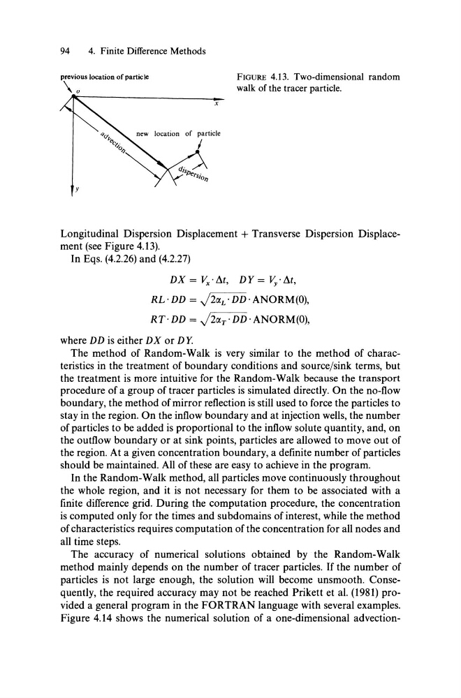
FIGURE 4.13. Two-dimensional random
walk of the tracer particle.
Longitudinal Dispersion Displacement + Transverse Dispersion Displacement (see Figure 4.13).
In Eqs. (4.2.26) and (4.2.27)
DX = v". M, DY = V,. M,
RL· DD = J2a. L • DD· ANORM(O),
RT·DD = J2a. T ·DD·ANORM(O),
where DD is either DX or DY.
The method of Random-Walk is very similar to the method of characteristics in the treatment of boundary conditions and source/sink terms, but
the treatment is more intuitive for the Random-Walk because the transport
procedure of a group of tracer particles is simulated directly. On the no-flow
boundary, the method of mirror reflection is still used to force the particles to
stay in the region. On the inflow boundary and at injection wells, the number
of particles to be added is proportional to the inflow solute quantity, and, on
the outflow boundary or at sink points, particles are allowed to move out of
the region. At a given concentration boundary, adefinite number of particles
should be maintained. All of these are easy to achieve in the program.
In the Random-Walk method, an particles move continuously throughout
the whole region, and it is not necessary for them to be associated with a
finite difference grid. During the computation procedure, the concentration
is computed only for the times and subdomains of interest, while the method
of characteristics requires computation of the concentration for an nodes and
an time steps.
The accuracy of numerical solutions obtained by the Random-Walk
method mainly depends on the number of tracer particles. If the number of
particles is not large enough, the solution will become unsmooth. Consequently, the required accuracy may not be reached Prikett et al. (1981) provided a general program in the FORTRAN language with several examples.
Figure 4.14 shows the numerical solution of a one-dimensional advection-
4. Finite Difference Methods
previous locatioD ofparticle
\0
FIGURE 4.13. Two-dimensional random
walk of the tracer particle.
Longitudinal Dispersion Displacement + Transverse Dispersion Displacement (see Figure 4.13).
In Eqs. (4.2.26) and (4.2.27)
DX = v". M, DY = V,. M,
RL· DD = J2a. L • DD· ANORM(O),
RT·DD = J2a. T ·DD·ANORM(O),
where DD is either DX or DY.
The method of Random-Walk is very similar to the method of characteristics in the treatment of boundary conditions and source/sink terms, but
the treatment is more intuitive for the Random-Walk because the transport
procedure of a group of tracer particles is simulated directly. On the no-flow
boundary, the method of mirror reflection is still used to force the particles to
stay in the region. On the inflow boundary and at injection wells, the number
of particles to be added is proportional to the inflow solute quantity, and, on
the outflow boundary or at sink points, particles are allowed to move out of
the region. At a given concentration boundary, adefinite number of particles
should be maintained. All of these are easy to achieve in the program.
In the Random-Walk method, an particles move continuously throughout
the whole region, and it is not necessary for them to be associated with a
finite difference grid. During the computation procedure, the concentration
is computed only for the times and subdomains of interest, while the method
of characteristics requires computation of the concentration for an nodes and
an time steps.
The accuracy of numerical solutions obtained by the Random-Walk
method mainly depends on the number of tracer particles. If the number of
particles is not large enough, the solution will become unsmooth. Consequently, the required accuracy may not be reached Prikett et al. (1981) provided a general program in the FORTRAN language with several examples.
Figure 4.14 shows the numerical solution of a one-dimensional advection-