

Exercises
95
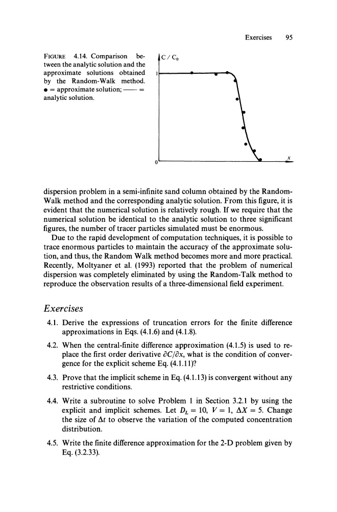
FIGURE 4.14. Comparison beC / Co
tween the analytic solution and the
approximate solutions obtained
by the Random-Walk method .
• = approximate solution; - - =
analytic solution.
o~-_ ________ ~ _____ x
dispersion problem in a semi-infinite sand column obtained by the RandomWalk method and the corresponding analytic solution. From this figure, it is
evident that the numerical solution is relatively rough. If we require that the
numerical solution be identical to the analytic solution to three significant
figures, the number of tracer partic1es simulated must be enormous.
Due to the rapid development of computation techniques, it is possible to
trace enormous partic1es to maintain the accuracy of the approximate solution, and thus, the Random Walk method becomes more and more practical.
Recently, Moltyaner et al. (1993) reported that the problem of numerical
dispersion was completely eliminated by using the Random-Talk method to
reproduce the observation results of a three-dimensional field experiment.
Exercises
4.1. Derive the expressions of truncation errors for the finite difTerence
approximations in Eqs. (4.1.6) and (4.1.8).
4.2. When the central-finite difTerence approximation (4.1.5) is used to replace the first order derivative fJCjfJx, what is the condition of convergence for the explicit scheme Eq. (4.1.11)?
4.3. Prove that the implicit scheme in Eq. (4.1.13) is convergent without any
restrictive conditions.
4.4. Write a subroutine to solve Problem 1 in Section 3.2.1 by using the
explicit and implicit schemes. Let D L = 10, V = 1, I!J.X = 5. Change
the size of ßt to observe the variation of the computed concentration
distribution.
4.5. Write the finite difTerence approximation for the 2-D problem given by
Eq. (3.2.33).
95
FIGURE 4.14. Comparison beC / Co
tween the analytic solution and the
approximate solutions obtained
by the Random-Walk method .
• = approximate solution; - - =
analytic solution.
o~-_ ________ ~ _____ x
dispersion problem in a semi-infinite sand column obtained by the RandomWalk method and the corresponding analytic solution. From this figure, it is
evident that the numerical solution is relatively rough. If we require that the
numerical solution be identical to the analytic solution to three significant
figures, the number of tracer partic1es simulated must be enormous.
Due to the rapid development of computation techniques, it is possible to
trace enormous partic1es to maintain the accuracy of the approximate solution, and thus, the Random Walk method becomes more and more practical.
Recently, Moltyaner et al. (1993) reported that the problem of numerical
dispersion was completely eliminated by using the Random-Talk method to
reproduce the observation results of a three-dimensional field experiment.
Exercises
4.1. Derive the expressions of truncation errors for the finite difTerence
approximations in Eqs. (4.1.6) and (4.1.8).
4.2. When the central-finite difTerence approximation (4.1.5) is used to replace the first order derivative fJCjfJx, what is the condition of convergence for the explicit scheme Eq. (4.1.11)?
4.3. Prove that the implicit scheme in Eq. (4.1.13) is convergent without any
restrictive conditions.
4.4. Write a subroutine to solve Problem 1 in Section 3.2.1 by using the
explicit and implicit schemes. Let D L = 10, V = 1, I!J.X = 5. Change
the size of ßt to observe the variation of the computed concentration
distribution.
4.5. Write the finite difTerence approximation for the 2-D problem given by
Eq. (3.2.33).