

86
4. Finite Difference Methods
of the grid square that it occupies, e.g., if particle P is located in grid square
(i,j), its initial concentration is prescribed to be Cp,o = Ci,i,O'
Our problem is how to determine the concentration of each grid square
corresponding to aseries of discrete instants in the future. The concentrations at aIl nodes are determined by both advection and dispersion effects.
According to the basic idea of the method of characteristics mentioned in
the previous paragraph, the two effects can be computed separately, where
the advection part may be computed by tracing the particle positions. It
is assumed that the concentration of any particle P at time t k is known as
Cp,k' its position is (Xp,k'YP,k)' and its velocity components are v",p,k and
Vy,p,k'
The position of particle P at tk+l = t k + I1t can be calculated approximatelyas
Xp,k+l = Xp,k + Vx,P,k 'l1t,
Y p,k+l = Yp,k + Vy,p,k ·l1t.
(4.2.7)
(4.2.8)
In fact, it is equivalent to using the simple method ofbroken lines to approximately solve the characteristics of Eqs. (4.2.3) and (4.2.4). The velocity components in the equations are easily determined based on the given flow field.
In terms of the flow field at a given time t k , the node values of velocity
components v",i,i,k and Vy,i,i,k can be obtained from Darcy's law. Ifparticle P
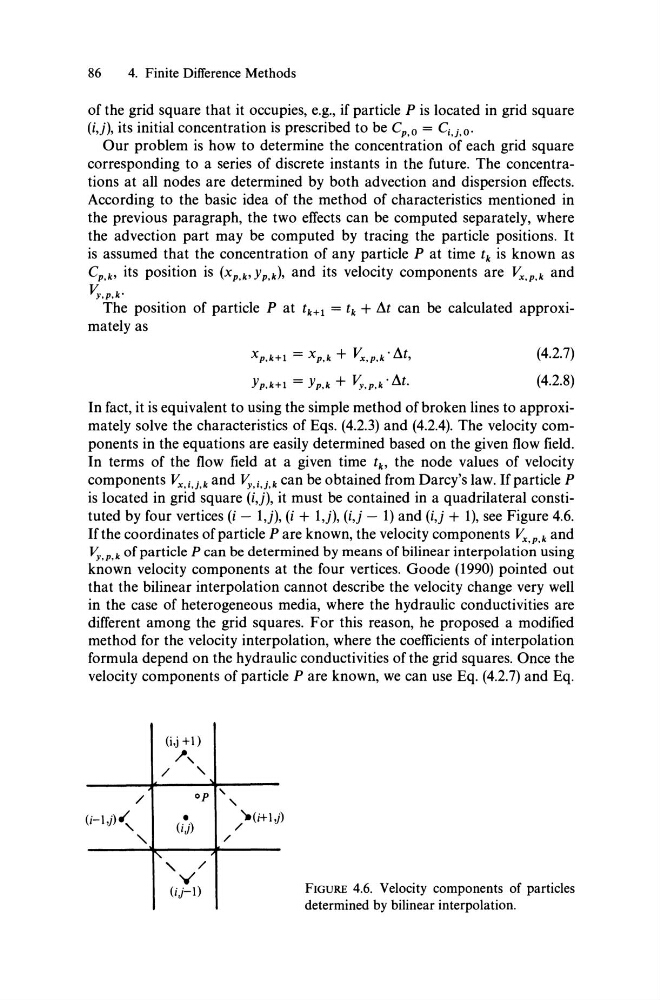
is located in grid square (i,j), it must be contained in a quadrilateral constituted by four vertices (i - l,j), (i + l,j), (i,j - 1) and (i,j + 1), see Figure 4.6.
If the coordinates of particle P are known, the velocity components Vx,p,k and
lj,p,k ofparticle P can be determined by means ofbilinear interpolation using
known velocity components at the four vertices. Goode (1990) pointed out
that the bilinear interpolation cannot describe the velocity change very weIl
in the case of heterogeneous media, where the hydraulic conductivities are
different among the grid squares. For this reason, he proposed a modified
method for the velocity interpolation, where the coefficients of interpolation
formula depend on the hydraulic conductivities of the grid squares. Once the
velocity components ofparticle P are known, we can use Eq. (4.2.7) and Eq.
(i,j +1)
1\
/
"
op , ,
•
'»(i+1,j)
(ij)
/
1", /
V
(ij-I)
/
FIGURE 4.6. Velocity components of particles
determined by bilinear interpolation.
4. Finite Difference Methods
of the grid square that it occupies, e.g., if particle P is located in grid square
(i,j), its initial concentration is prescribed to be Cp,o = Ci,i,O'
Our problem is how to determine the concentration of each grid square
corresponding to aseries of discrete instants in the future. The concentrations at aIl nodes are determined by both advection and dispersion effects.
According to the basic idea of the method of characteristics mentioned in
the previous paragraph, the two effects can be computed separately, where
the advection part may be computed by tracing the particle positions. It
is assumed that the concentration of any particle P at time t k is known as
Cp,k' its position is (Xp,k'YP,k)' and its velocity components are v",p,k and
Vy,p,k'
The position of particle P at tk+l = t k + I1t can be calculated approximatelyas
Xp,k+l = Xp,k + Vx,P,k 'l1t,
Y p,k+l = Yp,k + Vy,p,k ·l1t.
(4.2.7)
(4.2.8)
In fact, it is equivalent to using the simple method ofbroken lines to approximately solve the characteristics of Eqs. (4.2.3) and (4.2.4). The velocity components in the equations are easily determined based on the given flow field.
In terms of the flow field at a given time t k , the node values of velocity
components v",i,i,k and Vy,i,i,k can be obtained from Darcy's law. Ifparticle P
is located in grid square (i,j), it must be contained in a quadrilateral constituted by four vertices (i - l,j), (i + l,j), (i,j - 1) and (i,j + 1), see Figure 4.6.
If the coordinates of particle P are known, the velocity components Vx,p,k and
lj,p,k ofparticle P can be determined by means ofbilinear interpolation using
known velocity components at the four vertices. Goode (1990) pointed out
that the bilinear interpolation cannot describe the velocity change very weIl
in the case of heterogeneous media, where the hydraulic conductivities are
different among the grid squares. For this reason, he proposed a modified
method for the velocity interpolation, where the coefficients of interpolation
formula depend on the hydraulic conductivities of the grid squares. Once the
velocity components ofparticle P are known, we can use Eq. (4.2.7) and Eq.
(i,j +1)
1\
/
"
op , ,
•
'»(i+1,j)
(ij)
/
1", /
V
(ij-I)
/
FIGURE 4.6. Velocity components of particles
determined by bilinear interpolation.