

4.2. The Method of Characteristics
85
dispersion terms, i.e.,
dC 0 (OC
OC) 0 (OC
OC)
Tl = OX Dxx OX + Dxy oy + oy Dxy oy + Dyy oy + I. (4.2.6)
The meaning of Eq. (4.2.6) is easily understood from the Lagrangian viewpoint. When we observe the process of advection-dispersion, not in a stationary coordinate system, but following a moving particle with an average
veiocity, what we see is not the advection, but only the dispersion in associati on with the particle. The solution of Eq. (4.2.6), C = C(t), represents the
time-dependent concentrations of the partieles moving along the characteristic. Therefore, if we set aseries of characteristics in the flow region, and find
the changes of concentration along these characteristics caused by dispersion effect only, then the advection-dispersion problem is solved under the
Lagrangian viewpoint. Since the solution under the Lagrangian viewpoint is
not intuitive, it is required to establish a fixed co ordinate system to describe
the space distribution of the concentration. A family of characteristics will be
depicted through a group of moving partieles in the fixed co ordinate system,
meanwhile the changes of concentrations of moving particles are transformed into the fixed nodes of finite difference. Thus, we can obtain the
conventional concentration distribution under the Eulerian viewpoint. In
this case, the method of characteristics (MOC), which will be stated in this
section, is actually a Lagrangian-Eulerian solution. The details of this technique will be presented in the following three sections.
4.2.2 Computation of the Advection Part
First, the domain being considered is divided into a common finite difference
grid. The initial concentrations at all nodes are determined according to the
given initial conditions. Let the initial concentration at node (i,j) be Ci,i,O'
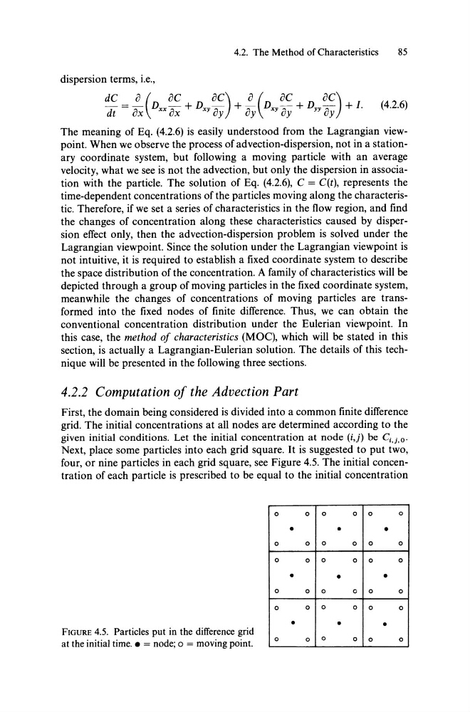
Next, place so me partieles into each grid square. It is suggested to put two,
four, or ni ne partieles in each grid square, see Figure 4.5. The initial concentration of each particle is prescribed to be equal to the initial concentration
FIGURE 4.5. Partieles put in the difference grid
at the initial time .• = node; 0 = moving point.
0
0
0
0
0
0
0
•
0
0
•
0
0
•
0
0
•
0
0
•
0
0
•
0
0
0
0
•
0
0
0
0
0
0
•
0
0
0
0
0
0
•
0
0
0
85
dispersion terms, i.e.,
dC 0 (OC
OC) 0 (OC
OC)
Tl = OX Dxx OX + Dxy oy + oy Dxy oy + Dyy oy + I. (4.2.6)
The meaning of Eq. (4.2.6) is easily understood from the Lagrangian viewpoint. When we observe the process of advection-dispersion, not in a stationary coordinate system, but following a moving particle with an average
veiocity, what we see is not the advection, but only the dispersion in associati on with the particle. The solution of Eq. (4.2.6), C = C(t), represents the
time-dependent concentrations of the partieles moving along the characteristic. Therefore, if we set aseries of characteristics in the flow region, and find
the changes of concentration along these characteristics caused by dispersion effect only, then the advection-dispersion problem is solved under the
Lagrangian viewpoint. Since the solution under the Lagrangian viewpoint is
not intuitive, it is required to establish a fixed co ordinate system to describe
the space distribution of the concentration. A family of characteristics will be
depicted through a group of moving partieles in the fixed co ordinate system,
meanwhile the changes of concentrations of moving particles are transformed into the fixed nodes of finite difference. Thus, we can obtain the
conventional concentration distribution under the Eulerian viewpoint. In
this case, the method of characteristics (MOC), which will be stated in this
section, is actually a Lagrangian-Eulerian solution. The details of this technique will be presented in the following three sections.
4.2.2 Computation of the Advection Part
First, the domain being considered is divided into a common finite difference
grid. The initial concentrations at all nodes are determined according to the
given initial conditions. Let the initial concentration at node (i,j) be Ci,i,O'
Next, place so me partieles into each grid square. It is suggested to put two,
four, or ni ne partieles in each grid square, see Figure 4.5. The initial concentration of each particle is prescribed to be equal to the initial concentration
FIGURE 4.5. Partieles put in the difference grid
at the initial time .• = node; 0 = moving point.
0
0
0
0
0
0
0
•
0
0
•
0
0
•
0
0
•
0
0
•
0
0
•
0
0
0
0
•
0
0
0
0
0
0
•
0
0
0
0
0
0
•
0
0
0