

45
un
+ un
n
n
n
At (1+112./+112
1+112.1-112 - U1_1!2.;+112 - Ui-I12.j_I/2
1] .. - '-'
I,j
2 t..x
n
n
n
n
+ Vi+1I2.j+1I2 + vi_I12.j+l12 - v i+ 1I2 ,j_112 - vi_112.j_1(2)
(14)
2 !'J.y
un
un
v~ .
- v~ .
1]~+1 =
n _ M ( i+112.; - i-l/2.; + 1,/+1/2
/./-112)
(15)
I,j
1]iJ
t..x
!'J.y
for the Band C grid, respectively,
y, v
t
1)
u
(i - 1(2. j + 1(2)
(i+ Ifl,j+ 1(2)
A grid: (i. j)
(i. j)
(i,j)
B grid: (i, j) (i-112,j-l/2) (i-I/2,j-112)
C grid: (i,j)
(i-I/2,J)
(i,j-112)
•
D grid: (i, j)
(i,j-112)
(i-I/2.J)
(i.J)
' - - - - - . - . . . (i+ 1(2,j-I/2)---- X, U
(i-112.j-l/2) ~"_-----i""'1
~x
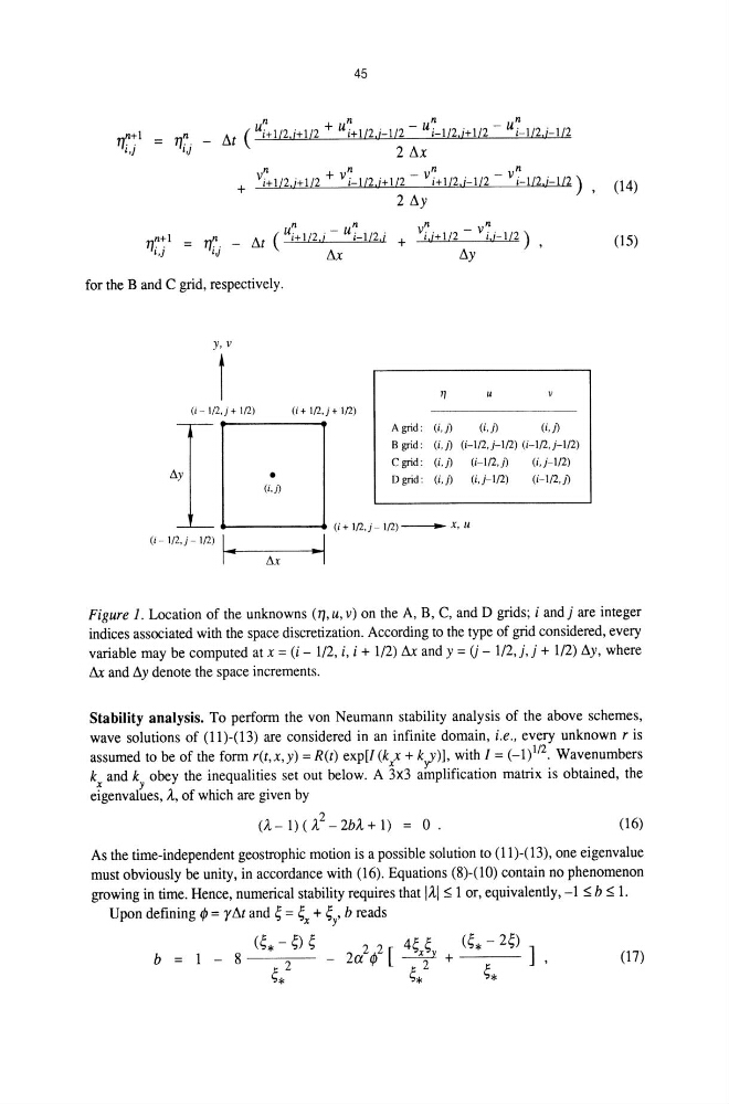
Figure 1. Location of the unknowns (1], u, v) on the A, B, C, and D grids; i and} are integer
indices associated with the space discretization. According to the type of grid considered, every
variable may be computed at x = (i - 1/2, i, i + 1/2) t..x and y = (j - 1/2,),} + 1/2) !'J.y, where
& and l'1y denote the space increments,
Stability analysis. To perform the von Neumann stability analysis of the above schemes,
wave solutions of (11)-(13) are considered in an infinite domain, i.e" every unknown r is
assumed to be of the form r(t,x,y) = R(t) exp[l (kxx + k;)], with I = (_1)112. Wavenumbers
k and k obey the inequalities set out below. A 3x3 amplification matrix is obtained, the
x
y
eigenvalues, A, of which are given by
(A-1)(A 2 -2bA+1) = O.
(16)
As the time-independent geostrophic motion is a possible solution to (11)-(13), one eigenvalue
must obviously be unity, in accordance with (16). Equations (8)-(10) contain no phenomenon
growing in time. Hence, numerical stability requires that 1.11:::; lor, equivalently, -1:::; b:::; 1.
Upon defining ¢ = yt..t and ~ = ~ + ~ , breads
x
y
(~*-~)~
(17)
un
+ un
n
n
n
At (1+112./+112
1+112.1-112 - U1_1!2.;+112 - Ui-I12.j_I/2
1] .. - '-'
I,j
2 t..x
n
n
n
n
+ Vi+1I2.j+1I2 + vi_I12.j+l12 - v i+ 1I2 ,j_112 - vi_112.j_1(2)
(14)
2 !'J.y
un
un
v~ .
- v~ .
1]~+1 =
n _ M ( i+112.; - i-l/2.; + 1,/+1/2
/./-112)
(15)
I,j
1]iJ
t..x
!'J.y
for the Band C grid, respectively,
y, v
t
1)
u
(i - 1(2. j + 1(2)
(i+ Ifl,j+ 1(2)
A grid: (i. j)
(i. j)
(i,j)
B grid: (i, j) (i-112,j-l/2) (i-I/2,j-112)
C grid: (i,j)
(i-I/2,J)
(i,j-112)
•
D grid: (i, j)
(i,j-112)
(i-I/2.J)
(i.J)
' - - - - - . - . . . (i+ 1(2,j-I/2)---- X, U
(i-112.j-l/2) ~"_-----i""'1
~x
Figure 1. Location of the unknowns (1], u, v) on the A, B, C, and D grids; i and} are integer
indices associated with the space discretization. According to the type of grid considered, every
variable may be computed at x = (i - 1/2, i, i + 1/2) t..x and y = (j - 1/2,),} + 1/2) !'J.y, where
& and l'1y denote the space increments,
Stability analysis. To perform the von Neumann stability analysis of the above schemes,
wave solutions of (11)-(13) are considered in an infinite domain, i.e" every unknown r is
assumed to be of the form r(t,x,y) = R(t) exp[l (kxx + k;)], with I = (_1)112. Wavenumbers
k and k obey the inequalities set out below. A 3x3 amplification matrix is obtained, the
x
y
eigenvalues, A, of which are given by
(A-1)(A 2 -2bA+1) = O.
(16)
As the time-independent geostrophic motion is a possible solution to (11)-(13), one eigenvalue
must obviously be unity, in accordance with (16). Equations (8)-(10) contain no phenomenon
growing in time. Hence, numerical stability requires that 1.11:::; lor, equivalently, -1:::; b:::; 1.
Upon defining ¢ = yt..t and ~ = ~ + ~ , breads
x
y
(~*-~)~
(17)