18
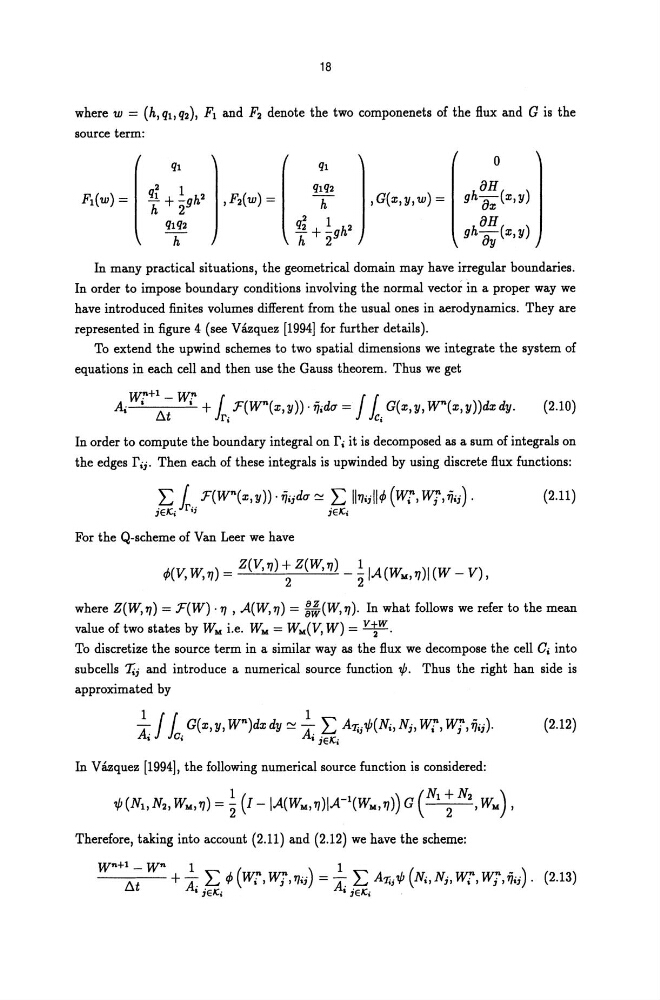
where w = (h,qt,q2), Fl and F2 denote the two componenets of the flux and G is the
source term:
o
aH
gha;(x,y)
aH
gh ay (x,y)
In many practical situations, the geometrical domain may have irregular boundaries.
In order to impose boundary conditions involving the normal vector in a proper way we
have introduced finites volumes different from the usual ones in aerodynamics. They are
represented in figure 4 (see Vazquez [1994] for further details).
To extend the upwind schemes to two spatial dimensions we integrate the system of
equations in each cell and then use the Gauss theorem. Thus we get
wn+1_ w~ 1
J
A; • b.
• + F(W"(x,y))·'Ij;du= (G(x,y,W"(x,y))dxdy.
t
ri
lei
(2.10)
In order to compute the boundary integral on r; it is decomposed as a sum of integrals on
the edges r;j. Then each of these integrals is upwinded by using discrete flux functions:
(2.11)
For the Q-scheme of Van Leer we have
where Z(W, 71) = F(W) . 71 , A(W, 71) = ::(W, 71). In what follows we refer to the mean
value of two states by WM i.e. WM = WM(V, W) = V ~w.
To discretize the source term in a similar way as the flux we decompose the cell C; into
sub cells T;j and introduce a numerical source function"p. Thus the right han side is
approximated by
(2.12)
In Vazquez [1994], the following numerical source function is considered:
Therefore, taking into account (2.11) and (2.12) we have the scheme: