

19
2.2 Numerical results
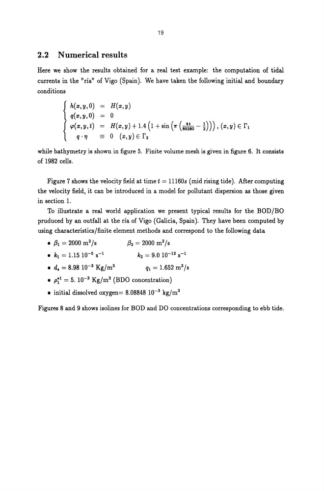
Here we show the results obtained for a real test example: the computation of tidal
currents in the "rla" of Vigo (Spain). We have taken the following initial and boundary
conditions
l
h(z,y,O)
q(z,y,O)
",(z, y, t)
q . ."
H(z,y)
o
H(x,y) + 1.4 (1 + sin (71" (8:2~ - ~))), (x,y) E r l
o (X,y)Er2
while bathymetry is shown in figure 5. Finite volume mesh is given in figure 6. It consists
of 1982 cells.
Figure 7 shows the velocity field at time t = 111608 (mid rising tide). After computing
the velocity field, it can be introduced in a model for pollutant dispersion as those given
in section 1.
To illustrate a real world application we present typical results for the BOD /BO
pruduced by an outfall at the rfa of Vigo (Galicia, Spain). They have been computed by
using characteristics/finite element methods and correspond to the following data
• (31 = 2000 m 2 /s
• k1 = 1.15 10- 5 5- 1
• d. = 8.98 10- 3 Kg/m 3
(32 = 2000 m 2 /s
k2 = 9.0 10- 12 5- 1
ql = 1.652 m 3 /s
• pi 1 = 5.10- 3 Kg/m 3 (BDO concentration)
• initial dissolved oxygen= 8.08848 10- 3 kg/m 3
Figures 8 and 9 shows isolines for BOD and DO concentrations corresponding to ebb tide.
2.2 Numerical results
Here we show the results obtained for a real test example: the computation of tidal
currents in the "rla" of Vigo (Spain). We have taken the following initial and boundary
conditions
l
h(z,y,O)
q(z,y,O)
",(z, y, t)
q . ."
H(z,y)
o
H(x,y) + 1.4 (1 + sin (71" (8:2~ - ~))), (x,y) E r l
o (X,y)Er2
while bathymetry is shown in figure 5. Finite volume mesh is given in figure 6. It consists
of 1982 cells.
Figure 7 shows the velocity field at time t = 111608 (mid rising tide). After computing
the velocity field, it can be introduced in a model for pollutant dispersion as those given
in section 1.
To illustrate a real world application we present typical results for the BOD /BO
pruduced by an outfall at the rfa of Vigo (Galicia, Spain). They have been computed by
using characteristics/finite element methods and correspond to the following data
• (31 = 2000 m 2 /s
• k1 = 1.15 10- 5 5- 1
• d. = 8.98 10- 3 Kg/m 3
(32 = 2000 m 2 /s
k2 = 9.0 10- 12 5- 1
ql = 1.652 m 3 /s
• pi 1 = 5.10- 3 Kg/m 3 (BDO concentration)
• initial dissolved oxygen= 8.08848 10- 3 kg/m 3
Figures 8 and 9 shows isolines for BOD and DO concentrations corresponding to ebb tide.