

321
where L is the latent heat.
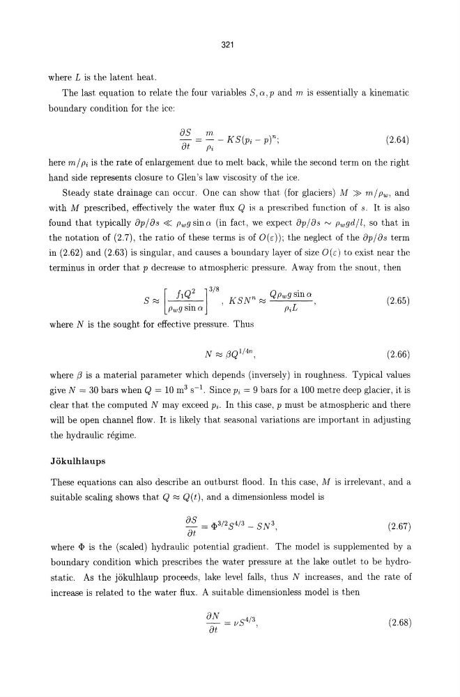
The last equation to relate the four variables S, a, P and m is essentially a kinematic
boundary condition for the ice:
as m
n
-
= - - K S(Pi - p) ;
at Pi
(2.64)
here m/ Pi is the rate of enlargement due to melt back, while the second term on the right
hand side represents closure to Glen's law viscosity of the ice.
Steady state drainage can occur. One can show that (for glaciers) M » m/ Pw, and
with M prescribed, effectively the water flux Q is a prescribed function of s. It is also
found that typically ap/as « pw9sina (in fact, we expect ap/os '" Pw9d/l, so that in
the notation of (2.7), the ratio of these terms is of 0(6)}; the neglect of the op/as term
in (2.62) and (2.63) is singular, and causes a boundary layer of size 0(6} to exist near the
terminus in order that p decrease t.o atmospheric pressure. Away from the snout, then
S f':j [ it ~2 ] 3/8, K S N n f':j Q Pw9 sin a ,
pw9sma
Pi L
(2.65)
where N is the sought for effective pressure. Thus
(2.66)
where (3 is a material parameter which depends (inversely) in roughness. Typical values
give N = 30 bars when Q = 10 m 3 s-l. Since Pi = 9 bars for a 100 metre deep glacier, it is
clear that the computed N may exceed Pi. In this case, p must be atmospheric and there
will be open channel flow. It is likely that seasonal variations are important in adjusting
the hydraulic regime.
Jokulhlaups
These equations can also describe an outburst flood. In this case, M is irrelevant, and a
suitable scaling shows that. Q f':j Q(t), and a dimensionless model is
(2.67)
where is the (scaled) hydraulic potent.ial gradient. The model is supplemented by a
boundary condition which prescribes the water pressure at the lake outlet to be hydrostatic. As the jokulhlaup proceeds, lake level falls, thus N increases, and the rate of
increase is related to the water flux. A suitable dimensionless model is then
aN = vS4/3
at
'
(2.68)
where L is the latent heat.
The last equation to relate the four variables S, a, P and m is essentially a kinematic
boundary condition for the ice:
as m
n
-
= - - K S(Pi - p) ;
at Pi
(2.64)
here m/ Pi is the rate of enlargement due to melt back, while the second term on the right
hand side represents closure to Glen's law viscosity of the ice.
Steady state drainage can occur. One can show that (for glaciers) M » m/ Pw, and
with M prescribed, effectively the water flux Q is a prescribed function of s. It is also
found that typically ap/as « pw9sina (in fact, we expect ap/os '" Pw9d/l, so that in
the notation of (2.7), the ratio of these terms is of 0(6)}; the neglect of the op/as term
in (2.62) and (2.63) is singular, and causes a boundary layer of size 0(6} to exist near the
terminus in order that p decrease t.o atmospheric pressure. Away from the snout, then
S f':j [ it ~2 ] 3/8, K S N n f':j Q Pw9 sin a ,
pw9sma
Pi L
(2.65)
where N is the sought for effective pressure. Thus
(2.66)
where (3 is a material parameter which depends (inversely) in roughness. Typical values
give N = 30 bars when Q = 10 m 3 s-l. Since Pi = 9 bars for a 100 metre deep glacier, it is
clear that the computed N may exceed Pi. In this case, p must be atmospheric and there
will be open channel flow. It is likely that seasonal variations are important in adjusting
the hydraulic regime.
Jokulhlaups
These equations can also describe an outburst flood. In this case, M is irrelevant, and a
suitable scaling shows that. Q f':j Q(t), and a dimensionless model is
(2.67)
where is the (scaled) hydraulic potent.ial gradient. The model is supplemented by a
boundary condition which prescribes the water pressure at the lake outlet to be hydrostatic. As the jokulhlaup proceeds, lake level falls, thus N increases, and the rate of
increase is related to the water flux. A suitable dimensionless model is then
aN = vS4/3
at
'
(2.68)