

291
ICE CAP MODEL OPERATING CURVE
1.0
0.9
0.8
I"al 0.7
~
0 .6
0 .5
0 0.4
~ 0 .3
0.2
0.1
0.0
300
360
400
460
600
Q (W/mZ)
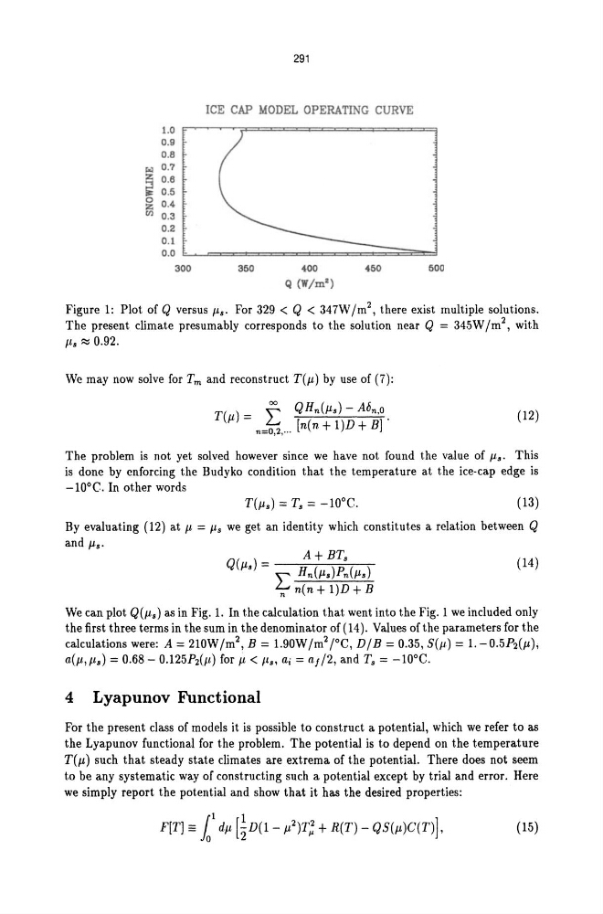
Figure 1: Plot of Q versus jl •. For 329 < Q < 347W 1m2, there exist multiple solut.ions.
The present climate presumably corresponds to the solution near Q = 345W 1m2, with
IL. ::::; 0.92.
We may now solve for Tm and reconstruct T(jl) by use of (7):
T(jl) = f QHn(Jl.) - Ac5n •o .
n =O.2 •. .. [n(n + 1)D + BJ
(12)
The problem is not yet solved however since we have not found the value of /1... This
is done by enforcing the Budyko condition t.hat the temperature at the ice-cap edge is
-lOoe. In other words
(13)
By evalua.ting (12) at /1, = /1" we get an identity which constitutes a relation between Q
and Jls.
Q(Jl.) =
A + BT.
E Hn(Jl.)Pn(Jl.)
nn(n+1}D+B
(14)
We can plot Q(/1.s) as in Fig. 1. In t.he calculation that. went into the Fig. 1 we included only
the first three terms in t.he sum in the denominator of (14). Values of the parameters for the
calculations were: A = 2lOW 1m2, B = 1.90W 1m2 re, D I B = 0.35, S(/1.) = 1. - 0.5P2(jl) ;
a(/1" Il.) = 0.68 - 0.125P2(ll) for Jl < Jt., aj = aJl2, and T. = - lOoe .
4 Lyapunov Functional
For the present class of models it is possible to construct a potential, which we refer to as
the Lyapunov functional for the problem. The potential is to depend on the temperature
T(Jl) such that steady state climates are extrema of the potential. There does not seem
to be any systematic way of constructing such a potential except by trial and error. Here
we simply report the potential and show that it has the desired properties:
(15)
ICE CAP MODEL OPERATING CURVE
1.0
0.9
0.8
I"al 0.7
~
0 .6
0 .5
0 0.4
~ 0 .3
0.2
0.1
0.0
300
360
400
460
600
Q (W/mZ)
Figure 1: Plot of Q versus jl •. For 329 < Q < 347W 1m2, there exist multiple solut.ions.
The present climate presumably corresponds to the solution near Q = 345W 1m2, with
IL. ::::; 0.92.
We may now solve for Tm and reconstruct T(jl) by use of (7):
T(jl) = f QHn(Jl.) - Ac5n •o .
n =O.2 •. .. [n(n + 1)D + BJ
(12)
The problem is not yet solved however since we have not found the value of /1... This
is done by enforcing the Budyko condition t.hat the temperature at the ice-cap edge is
-lOoe. In other words
(13)
By evalua.ting (12) at /1, = /1" we get an identity which constitutes a relation between Q
and Jls.
Q(Jl.) =
A + BT.
E Hn(Jl.)Pn(Jl.)
nn(n+1}D+B
(14)
We can plot Q(/1.s) as in Fig. 1. In t.he calculation that. went into the Fig. 1 we included only
the first three terms in t.he sum in the denominator of (14). Values of the parameters for the
calculations were: A = 2lOW 1m2, B = 1.90W 1m2 re, D I B = 0.35, S(/1.) = 1. - 0.5P2(jl) ;
a(/1" Il.) = 0.68 - 0.125P2(ll) for Jl < Jt., aj = aJl2, and T. = - lOoe .
4 Lyapunov Functional
For the present class of models it is possible to construct a potential, which we refer to as
the Lyapunov functional for the problem. The potential is to depend on the temperature
T(Jl) such that steady state climates are extrema of the potential. There does not seem
to be any systematic way of constructing such a potential except by trial and error. Here
we simply report the potential and show that it has the desired properties:
(15)