

where T/l = dT/dp,
292
R(T) = JT I(T') dT'
C(p, T) = JT a(p, T') dT'
(16)
(17)
where I(T) = A + BT, and we have chosen to write a(p., P.) as a function of p and T, e.g.,
a(p, T) = (ao + a2P2(p))(9(T - T.) + 0.59(Ts - T))
(18)
where 9(Z) is the unit step function, 9 = 0 for Z < 0, 9 = 1 for Z > o. We can examine
the funcional for an arbitrary small variation hT(p); i.e., T(p) is replaced by T(p) + hT(p)
to form F[T] + hF[T]. After subtracting F[T] we have
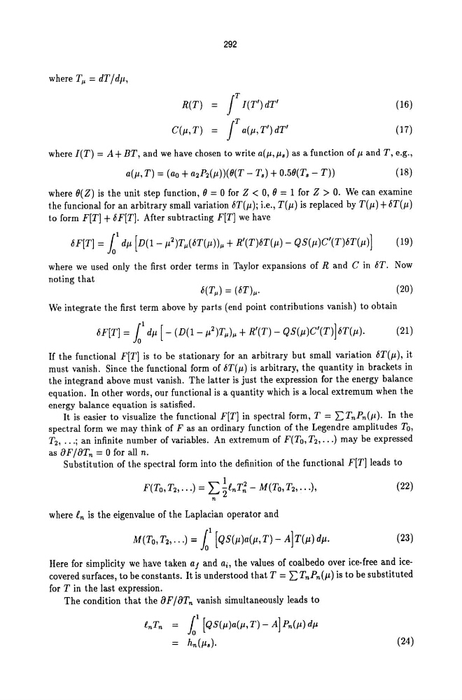
hF[T] = l dp [D(1_p2)T/l(hT(p))/l + R'(T)hT(p) - QS(ll)C'(T)hT(p)j (19)
where we used only the first order terms in Taylor expansions of Rand C in hT. Now
noting that
(20)
We integrate the first term a,bove by pa,rts (end point contributions vanish) to obtain
If the functional F[T] is to be stationary for an arbitrary but small variation hT(p), it
must vanish. Since the functional form of hT(Jl) is arbitrary, the quantity in brackets in
the integrand above must vanish. The latter is just the expression for the energy balance
equation. In other words, our functional is a quantity which is a local extremum when the
energy balance equation is satisfied.
It is easier to visualize the functional F[T] in spectral form, T = 'L,TnPn(Jt). In the
spectral form we may think of F as an ordinary function of the Legendre amplitudes To,
T2 , ••• ; an infinite number of variables. An extremum of F(To, T2 , ••• ) may be expressed
as {)F/{)Tn = 0 for all n.
Substitution of the spectral form into the definition of the functional F[T] leads to
(22)
where en is the eigenvalue of the Laplacian operator and
(23)
Here for simplicity we have taken af and ai, the values of coalbedo over ice-free and icecovered surfaces, to be constants. It is understood that T = 'L, TnPn(Jl) is to be substituted
for T in the last expression.
The condition that the {)F/{)Tn vanish simultaneously leads to
eSn
10
1 [QS(p)a(Jl, T) - A] Pn(P) dp
= hn{Jls).
(24)
292
R(T) = JT I(T') dT'
C(p, T) = JT a(p, T') dT'
(16)
(17)
where I(T) = A + BT, and we have chosen to write a(p., P.) as a function of p and T, e.g.,
a(p, T) = (ao + a2P2(p))(9(T - T.) + 0.59(Ts - T))
(18)
where 9(Z) is the unit step function, 9 = 0 for Z < 0, 9 = 1 for Z > o. We can examine
the funcional for an arbitrary small variation hT(p); i.e., T(p) is replaced by T(p) + hT(p)
to form F[T] + hF[T]. After subtracting F[T] we have
hF[T] = l dp [D(1_p2)T/l(hT(p))/l + R'(T)hT(p) - QS(ll)C'(T)hT(p)j (19)
where we used only the first order terms in Taylor expansions of Rand C in hT. Now
noting that
(20)
We integrate the first term a,bove by pa,rts (end point contributions vanish) to obtain
If the functional F[T] is to be stationary for an arbitrary but small variation hT(p), it
must vanish. Since the functional form of hT(Jl) is arbitrary, the quantity in brackets in
the integrand above must vanish. The latter is just the expression for the energy balance
equation. In other words, our functional is a quantity which is a local extremum when the
energy balance equation is satisfied.
It is easier to visualize the functional F[T] in spectral form, T = 'L,TnPn(Jt). In the
spectral form we may think of F as an ordinary function of the Legendre amplitudes To,
T2 , ••• ; an infinite number of variables. An extremum of F(To, T2 , ••• ) may be expressed
as {)F/{)Tn = 0 for all n.
Substitution of the spectral form into the definition of the functional F[T] leads to
(22)
where en is the eigenvalue of the Laplacian operator and
(23)
Here for simplicity we have taken af and ai, the values of coalbedo over ice-free and icecovered surfaces, to be constants. It is understood that T = 'L, TnPn(Jl) is to be substituted
for T in the last expression.
The condition that the {)F/{)Tn vanish simultaneously leads to
eSn
10
1 [QS(p)a(Jl, T) - A] Pn(P) dp
= hn{Jls).
(24)