

176
Ill.S Principle of the numerical resolution
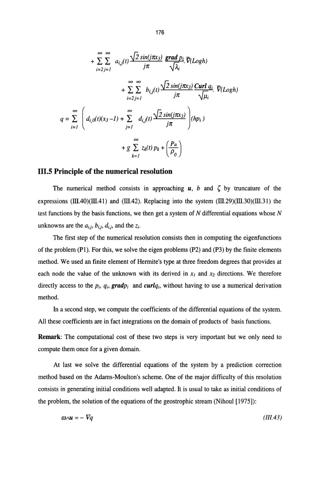
The numerical method consists in approaching u. b and ; by truncature of the
expressions (III.40)(III.41) and (III.42). Replacing into the system (III.29)(III.30)(III.31) the
test functions by the basis functions. we then get a system of N differential equations whose N
unknowns are the ai,j. bi,j. diJ• and the Zi.
The first step of the numerical resolution consists then in computing the eigenfunctions
of the problem (PI). For this. we solve the eigen problems (P2) and (P3) by the finite elements
method. We used an finite element of Hermite's type at three freedom degrees that provides at
each node the value of the unknown with its derived in XI and X2 directions. We therefore
directly access to the Pi. qi. grad Pi and curlq;, without having to use a numerical derivation
method.
In a second step. we compute the coefficients of the differential equations of the system.
All these coefficients are in fact integrations on the domain of products of basis functions.
Remark: The computational cost of these two steps is very important but we only need to
compute them once for a given domain.
At last we solve the differential equations of the system by a prediction correction
method based on the Adams-Moulton's scheme. One of the major difficulty of this resolution
consists in generating initial conditions well adapted. It is usual to take as initial conditions of
the problem. the solution of the equations of the geostrophic stream (Nihoul [1975]):
OJ"u =- Vq
(IIl.43 )
Ill.S Principle of the numerical resolution
The numerical method consists in approaching u. b and ; by truncature of the
expressions (III.40)(III.41) and (III.42). Replacing into the system (III.29)(III.30)(III.31) the
test functions by the basis functions. we then get a system of N differential equations whose N
unknowns are the ai,j. bi,j. diJ• and the Zi.
The first step of the numerical resolution consists then in computing the eigenfunctions
of the problem (PI). For this. we solve the eigen problems (P2) and (P3) by the finite elements
method. We used an finite element of Hermite's type at three freedom degrees that provides at
each node the value of the unknown with its derived in XI and X2 directions. We therefore
directly access to the Pi. qi. grad Pi and curlq;, without having to use a numerical derivation
method.
In a second step. we compute the coefficients of the differential equations of the system.
All these coefficients are in fact integrations on the domain of products of basis functions.
Remark: The computational cost of these two steps is very important but we only need to
compute them once for a given domain.
At last we solve the differential equations of the system by a prediction correction
method based on the Adams-Moulton's scheme. One of the major difficulty of this resolution
consists in generating initial conditions well adapted. It is usual to take as initial conditions of
the problem. the solution of the equations of the geostrophic stream (Nihoul [1975]):
OJ"u =- Vq
(IIl.43 )