

67
4-3 AVE RAG E ACCE LE RATION AN D I NSTANTAN EOUS ACCE LE RATION
(Answer)
and
(Answer)
Check: Is the angle Ϫ130° or Ϫ130° ϩ 180° ϭ 50°?
ϭ tan
Ϫ1
1.19 ϭ Ϫ130Њ.
ϭ tan
Ϫ1
v y
v x
ϭ tan
Ϫ1
Ϫ2.5 m /s
Ϫ2.1 m /s
ϭ 3.3 m /s
v ϭ 2v x
2 ϩ v y
2 ϭ 2(Ϫ2.1 m /s)
2 ϩ (Ϫ2.5 m /s)
2
For the rabbit in the preceding sample problem, find the
velocity at time t ϭ 15 s.
KEY IDEA
We can find by taking derivatives of the components of
the rabbit’s position vector.
Calculations: Applying the v x part of Eq. 4-12 to Eq. 4-5,
we find the x component of to be
(4-13)
At t ϭ 15 s, this gives v x ϭ Ϫ2.1 m/s. Similarly, applying the
v y part of Eq. 4-12 to Eq. 4-6, we find
(4-14)
At t ϭ 15 s, this gives v y ϭ Ϫ2.5 m/s. Equation 4-11 then yields
(Answer)
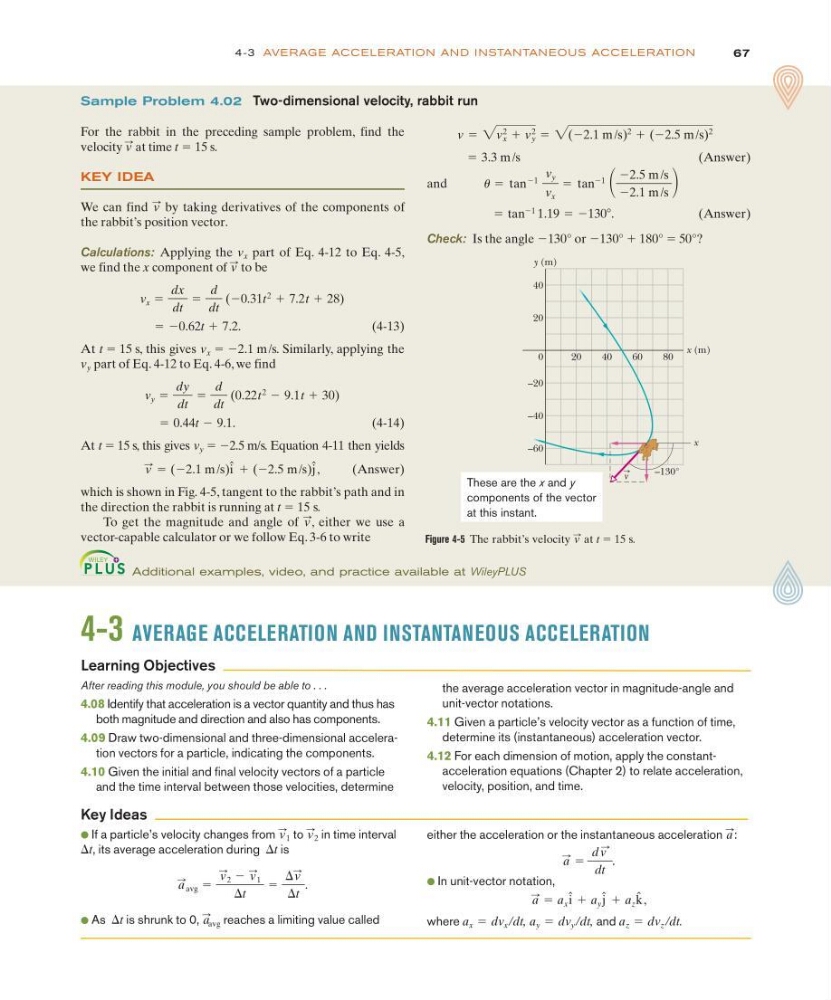
which is shown in Fig. 4-5, tangent to the rabbit’s path and in
the direction the rabbit is running at t ϭ 15 s.
To get the magnitude and angle of , either we use a
vector-capable calculator or we follow Eq. 3-6 to write
v
:
v
: ϭ (Ϫ2.1 m /s)i ˆ ϩ (Ϫ2.5 m /s)j ˆ ,
ϭ 0.44t Ϫ 9.1.
v y ϭ
dy
dt
ϭ
d
dt
(0.22t
2 Ϫ 9.1t ϩ 30)
ϭ Ϫ0.62t ϩ 7.2.
v x ϭ
dx
dt
ϭ
d
dt
(Ϫ0.31t
2 ϩ 7.2t ϩ 28)
v
:
v
:
v
:
Sample Problem 4.02 Two-dimensional velocity, rabbit run
Additional examples, video, and practice available at WileyPLUS
Figure 4-5 The rabbit’s velocity at t ϭ 15 s.
v
:
–130°
x (m)
0
20
40
–20
–40
–60
y (m)
20
40
60
80
x
v
These are the x and y
components of the vector
at this instant.
4-3 AVERAGE ACCELERATION AND INSTANTANEOUS ACCELERATION
the average acceleration vector in magnitude-angle and
unit-vector notations.
4.11 Given a particle’s velocity vector as a function of time,
determine its (instantaneous) acceleration vector.
4.12 For each dimension of motion, apply the constantacceleration equations (Chapter 2) to relate acceleration,
velocity, position, and time.
Learning Objectives
After reading this module, you should be able to . . .
4.08 Identify that acceleration is a vector quantity and thus has
both magnitude and direction and also has components.
4.09 Draw two-dimensional and three-dimensional acceleration vectors for a particle, indicating the components.
4.10 Given the initial and final velocity vectors of a particle
and the time interval between those velocities, determine
either the acceleration or the instantaneous acceleration :
● In unit-vector notation,
where
and a z ϭ dv z /dt.
a x ϭ dv x /dt, a y ϭ dv y /dt,
a
: ϭ a x i ˆ ϩ a y j ˆ ϩ a z k ˆ ,
a
: ϭ
d v
:
dt
.
a
:
Key Ideas
● If a particle’s velocity changes from to in time interval
t, its average acceleration during t is
● As t is shrunk to 0,
reaches a limiting value called
a
:
avg
⌬
a
:
avg ϭ
v
:
2 Ϫ v
:
1
⌬t
ϭ
⌬v
:
⌬t
.
⌬
⌬
v
:
2
v
:
1
4-3 AVE RAG E ACCE LE RATION AN D I NSTANTAN EOUS ACCE LE RATION
(Answer)
and
(Answer)
Check: Is the angle Ϫ130° or Ϫ130° ϩ 180° ϭ 50°?
ϭ tan
Ϫ1
1.19 ϭ Ϫ130Њ.
ϭ tan
Ϫ1
v y
v x
ϭ tan
Ϫ1
Ϫ2.5 m /s
Ϫ2.1 m /s
ϭ 3.3 m /s
v ϭ 2v x
2 ϩ v y
2 ϭ 2(Ϫ2.1 m /s)
2 ϩ (Ϫ2.5 m /s)
2
For the rabbit in the preceding sample problem, find the
velocity at time t ϭ 15 s.
KEY IDEA
We can find by taking derivatives of the components of
the rabbit’s position vector.
Calculations: Applying the v x part of Eq. 4-12 to Eq. 4-5,
we find the x component of to be
(4-13)
At t ϭ 15 s, this gives v x ϭ Ϫ2.1 m/s. Similarly, applying the
v y part of Eq. 4-12 to Eq. 4-6, we find
(4-14)
At t ϭ 15 s, this gives v y ϭ Ϫ2.5 m/s. Equation 4-11 then yields
(Answer)
which is shown in Fig. 4-5, tangent to the rabbit’s path and in
the direction the rabbit is running at t ϭ 15 s.
To get the magnitude and angle of , either we use a
vector-capable calculator or we follow Eq. 3-6 to write
v
:
v
: ϭ (Ϫ2.1 m /s)i ˆ ϩ (Ϫ2.5 m /s)j ˆ ,
ϭ 0.44t Ϫ 9.1.
v y ϭ
dy
dt
ϭ
d
dt
(0.22t
2 Ϫ 9.1t ϩ 30)
ϭ Ϫ0.62t ϩ 7.2.
v x ϭ
dx
dt
ϭ
d
dt
(Ϫ0.31t
2 ϩ 7.2t ϩ 28)
v
:
v
:
v
:
Sample Problem 4.02 Two-dimensional velocity, rabbit run
Additional examples, video, and practice available at WileyPLUS
Figure 4-5 The rabbit’s velocity at t ϭ 15 s.
v
:
–130°
x (m)
0
20
40
–20
–40
–60
y (m)
20
40
60
80
x
v
These are the x and y
components of the vector
at this instant.
4-3 AVERAGE ACCELERATION AND INSTANTANEOUS ACCELERATION
the average acceleration vector in magnitude-angle and
unit-vector notations.
4.11 Given a particle’s velocity vector as a function of time,
determine its (instantaneous) acceleration vector.
4.12 For each dimension of motion, apply the constantacceleration equations (Chapter 2) to relate acceleration,
velocity, position, and time.
Learning Objectives
After reading this module, you should be able to . . .
4.08 Identify that acceleration is a vector quantity and thus has
both magnitude and direction and also has components.
4.09 Draw two-dimensional and three-dimensional acceleration vectors for a particle, indicating the components.
4.10 Given the initial and final velocity vectors of a particle
and the time interval between those velocities, determine
either the acceleration or the instantaneous acceleration :
● In unit-vector notation,
where
and a z ϭ dv z /dt.
a x ϭ dv x /dt, a y ϭ dv y /dt,
a
: ϭ a x i ˆ ϩ a y j ˆ ϩ a z k ˆ ,
a
: ϭ
d v
:
dt
.
a
:
Key Ideas
● If a particle’s velocity changes from to in time interval
t, its average acceleration during t is
● As t is shrunk to 0,
reaches a limiting value called
a
:
avg
⌬
a
:
avg ϭ
v
:
2 Ϫ v
:
1
⌬t
ϭ
⌬v
:
⌬t
.
⌬
⌬
v
:
2
v
:
1