

701
24-6 CALCU L ATI NG TH E FI E LD FROM TH E POTE NTIAL
Calculating the Field from the Potential
In Module 24-2, you saw how to find the potential at a point f if you know
the electric field along a path from a reference point to point f. In this module,
we propose to go the other way — that is, to find the electric field when we know
the potential. As Fig. 24-5 shows, solving this problem graphically is easy: If we
know the potential V at all points near an assembly of charges, we can draw in
a family of equipotential surfaces. The electric field lines, sketched perpendicular
to those surfaces, reveal the variation of . What we are seeking here is the mathematical equivalent of this graphical procedure.
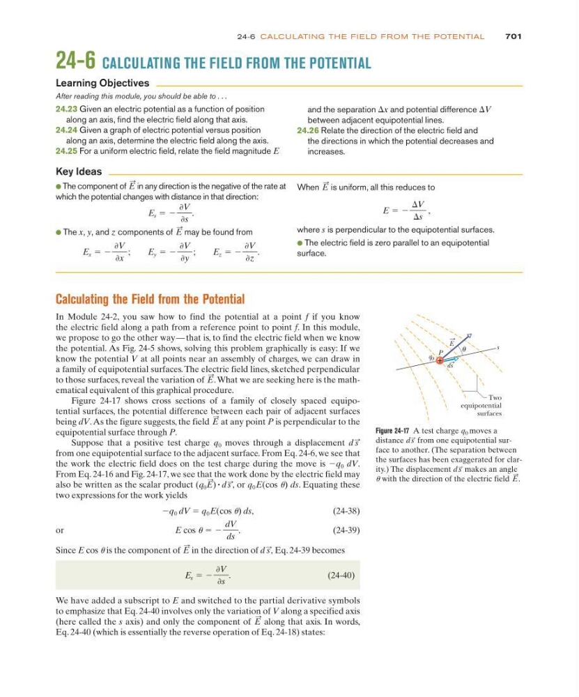
Figure 24-17 shows cross sections of a family of closely spaced equipotential surfaces, the potential difference between each pair of adjacent surfaces
being dV. As the figure suggests, the field at any point P is perpendicular to the
equipotential surface through P.
Suppose that a positive test charge q 0 moves through a displacement
from one equipotential surface to the adjacent surface. From Eq. 24-6, we see that
the work the electric field does on the test charge during the move is Ϫq 0 dV.
From Eq. 24-16 and Fig. 24-17, we see that the work done by the electric field may
also be written as the scalar product
or q 0 E(cos u) ds. Equating these
two expressions for the work yields
Ϫq 0 dV ϭ q 0 E(cos u) ds,
( 2 4 - 3 8 )
or
(24-39)
Since E cos u is the component of in the direction of
Eq. 24-39 becomes
(24-40)
We have added a subscript to E and switched to the partial derivative symbols
to emphasize that Eq. 24-40 involves only the variation of V along a specified axis
(here called the s axis) and only the component of
along that axis. In words,
Eq. 24-40 (which is essentially the reverse operation of Eq. 24-18) states:
E
:
E s ϭ Ϫ
ѨV
Ѩs
.
d s
:
,
E
:
E cos u ϭ Ϫ
dV
ds
.
(q 0 E
:
) ؒ d s
:
,
d s
:
E
:
E
:
s
q 0
P
θ
Two
equipotential
surfaces
+ ds
E
Figure 24-17 A test charge q 0 moves a
distance
from one equipotential surface to another. (The separation between
the surfaces has been exaggerated for clarity.) The displacement
makes an angle
u with the direction of the electric field .
E
:
d s
:
d s
:
24-6 CALCULATING THE FIELD FROM THE POTENTIAL
After reading this module, you should be able to . . .
24.23 Given an electric potential as a function of position
along an axis, find the electric field along that axis.
24.24 Given a graph of electric potential versus position
along an axis, determine the electric field along the axis.
24.25 For a uniform electric field, relate the field magnitude E
and the separation x and potential difference V
between adjacent equipotential lines.
24.26 Relate the direction of the electric field and
the directions in which the potential decreases and
increases.
⌬
⌬
Learning Objectives
● The component of in any direction is the negative of the rate at
which the potential changes with distance in that direction:
● The x, y, and z components of may be found from
E x ϭ Ϫ
ѨV
Ѩx
;
E y ϭ Ϫ
ѨV
Ѩy
;
E z ϭ Ϫ
ѨV
Ѩz
.
E
:
E s ϭ Ϫ
ѨV
Ѩs
.
E
:
When is uniform, all this reduces to
where s is perpendicular to the equipotential surfaces.
● The electric field is zero parallel to an equipotential
surface.
E ϭ Ϫ
⌬V
⌬s
,
E
:
Key Ideas