

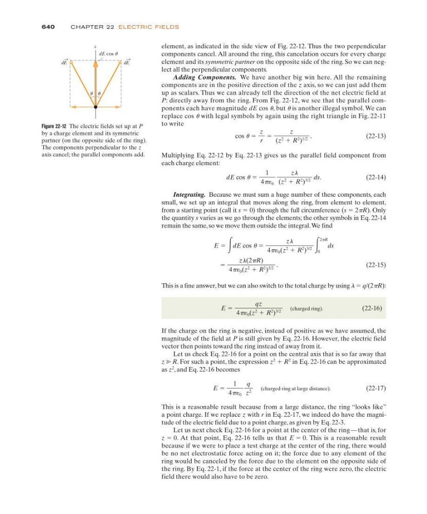
element, as indicated in the side view of Fig. 22-12. Thus the two perpendicular
components cancel. All around the ring, this cancelation occurs for every charge
element and its symmetric partner on the opposite side of the ring. So we can neglect all the perpendicular components.
Adding Components. We have another big win here. All the remaining
components are in the positive direction of the z axis, so we can just add them
up as scalars. Thus we can already tell the direction of the net electric field at
P: directly away from the ring. From Fig. 22-12, we see that the parallel components each have magnitude dE cos u, but u is another illegal symbol. We can
replace cos u with legal symbols by again using the right triangle in Fig. 22-11
to write
(22-13)
Multiplying Eq. 22-12 by Eq. 22-13 gives us the parallel field component from
each charge element:
(22-14)
Integrating. Because we must sum a huge number of these components, each
small, we set up an integral that moves along the ring, from element to element,
from a starting point (call it s ϭ 0) through the full circumference (s ϭ 2pR). Only
the quantity s varies as we go through the elements; the other symbols in Eq. 22-14
remain the same, so we move them outside the integral.We find
(22-15)
This is a fine answer, but we can also switch to the total charge by using l ϭ q/(2pR):
(charged ring).
(22-16)
If the charge on the ring is negative, instead of positive as we have assumed, the
magnitude of the field at P is still given by Eq. 22-16. However, the electric field
vector then points toward the ring instead of away from it.
Let us check Eq. 22-16 for a point on the central axis that is so far away that
z ӷ R. For such a point, the expression z
2 ϩ R
2
in Eq. 22-16 can be approximated
as z
2
, and Eq. 22-16 becomes
(charged ring at large distance).
(22-17)
This is a reasonable result because from a large distance, the ring “looks like”
a point charge. If we replace z with r in Eq. 22-17, we indeed do have the magnitude of the electric field due to a point charge, as given by Eq. 22-3.
Let us next check Eq. 22-16 for a point at the center of the ring — that is, for
z ϭ 0. At that point, Eq. 22-16 tells us that E ϭ 0. This is a reasonable result
because if we were to place a test charge at the center of the ring, there would
be no net electrostatic force acting on it; the force due to any element of the
ring would be canceled by the force due to the element on the opposite side of
the ring. By Eq. 22-1, if the force at the center of the ring were zero, the electric
field there would also have to be zero.
E ϭ
1
4p´ 0
q
z
2
E ϭ
qz
4p´ 0 (z
2 ϩ R
2
)
3/2
ϭ
zl(2pR)
4p´ 0 (z
2 ϩ R
2
)
3/2
.
E ϭ ͵dE cos u ϭ
zl
4p´ 0 (z
2 ϩ R
2
)
3/2 ͵
2pR
0
ds
dE cos u ϭ
1
4p 0
zl
(z
2 ϩ R
2
)
3/2
ds.
cos u ϭ
z
r
ϭ
z
(z
2 ϩ R
2
)
1/2
.
640
CHAPTE R 22 ELECTRIC FIELDS
z
dE cos u
u u
dE
dE
Figure 22-12 The electric fields set up at P
by a charge element and its symmetric
partner (on the opposite side of the ring).
The components perpendicular to the z
axis cancel; the parallel components add.