

639
22-4 TH E E LECTR IC FI E LD DU E TO A LI N E OF CHARG E
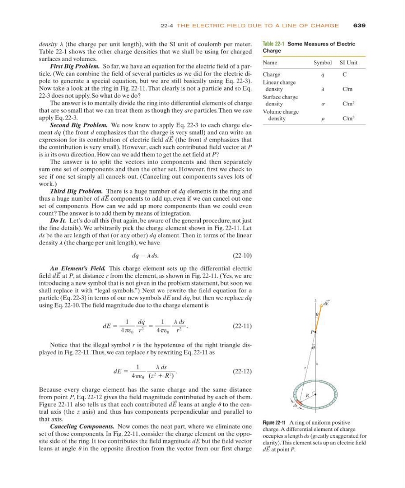
Figure 22-11 A ring of uniform positive
charge. A differential element of charge
occupies a length ds (greatly exaggerated for
clarity).This element sets up an electric field
at point P.
dE
:
+
+
+
+
+
+
+
+
+
+
+
+
+
+ + +
+ + + + +
+
+
+
+
+
+
+
+
+
z
ds
R
r
θ
θ
P
z
dE
density l (the charge per unit length), with the SI unit of coulomb per meter.
Table 22-1 shows the other charge densities that we shall be using for charged
surfaces and volumes.
First Big Problem. So far, we have an equation for the electric field of a particle. (We can combine the field of several particles as we did for the electric dipole to generate a special equation, but we are still basically using Eq. 22-3).
Now take a look at the ring in Fig. 22-11. That clearly is not a particle and so Eq.
22-3 does not apply. So what do we do?
The answer is to mentally divide the ring into differential elements of charge
that are so small that we can treat them as though they are particles. Then we can
apply Eq. 22-3.
Second Big Problem. We now know to apply Eq. 22-3 to each charge element dq (the front d emphasizes that the charge is very small) and can write an
expression for its contribution of electric field
(the front d emphasizes that
the contribution is very small). However, each such contributed field vector at P
is in its own direction. How can we add them to get the net field at P?
The answer is to split the vectors into components and then separately
sum one set of components and then the other set. However, first we check to
see if one set simply all cancels out. (Canceling out components saves lots of
work.)
Third Big Problem. There is a huge number of dq elements in the ring and
thus a huge number of
components to add up, even if we can cancel out one
set of components. How can we add up more components than we could even
count? The answer is to add them by means of integration.
Do It. Let’s do all this (but again, be aware of the general procedure, not just
the fine details). We arbitrarily pick the charge element shown in Fig. 22-11. Let
ds be the arc length of that (or any other) dq element. Then in terms of the linear
density l (the charge per unit length), we have
dq ϭ l ds.
( 2 2 - 1 0 )
An Element’s Field. This charge element sets up the differential electric
field
at P, at distance r from the element, as shown in Fig. 22-11. (Yes, we are
introducing a new symbol that is not given in the problem statement, but soon we
shall replace it with “legal symbols.”) Next we rewrite the field equation for a
particle (Eq. 22-3) in terms of our new symbols dE and dq, but then we replace dq
using Eq. 22-10. The field magnitude due to the charge element is
(22-11)
Notice that the illegal symbol r is the hypotenuse of the right triangle displayed in Fig. 22-11. Thus, we can replace r by rewriting Eq. 22-11 as
(22-12)
Because every charge element has the same charge and the same distance
from point P, Eq. 22-12 gives the field magnitude contributed by each of them.
Figure 22-11 also tells us that each contributed
leans at angle u to the central axis (the z axis) and thus has components perpendicular and parallel to
that axis.
Canceling Components. Now comes the neat part, where we eliminate one
set of those components. In Fig. 22-11, consider the charge element on the opposite side of the ring. It too contributes the field magnitude dE but the field vector
leans at angle u in the opposite direction from the vector from our first charge
dE
:
dE ϭ
1
4p´ 0
l ds
(z
2 ϩ R
2
)
.
dE ϭ
1
4p´ 0
dq
r
2
ϭ
1
4p´ 0
l ds
r
2
.
dE
:
dE
:
dE
:
Table 22-1 Some Measures of Electric
Charge
Name
Symbol SI Unit
Charge
q
C
Linear charge
density
l
C/m
Surface charge
density
s
C/m
2
Volume charge
density
r
C/m
3