

641
22-4 TH E E LECTR IC FI E LD DU E TO A LI N E OF CHARG E
Sample Problem 22.03 Electric field of a charged circular rod
60°
60°
P
y
x
r
Plastic rod
of charge –Q
(a)
This negatively charged rod
is obviously not a particle.
P
y
x
(g )
θ
ds
r
d
We use this to
relate the element’s
arc length to the
angle that it subtends.
x
P
y
(e)
θ
θ
ds
dE y
Symmetric
element ds'
dE
dE'
These y components just
cancel, so neglect them.
P
y
x
(b)
ds
But we can treat this
element as a particle.
Here is the field created by
the symmetric element, same
size and angle.
P
y
x
(d)
θ
θ
ds
Symmetric
element ds'
dE
dE'
P
y
x
(c)
θ
ds
dE
Here is the field the
element creates.
x
P
y
( f )
θ
θ
ds
dE x
Symmetric
element ds'
dE
dE'
These x components add.
Our job is to add all such
components.
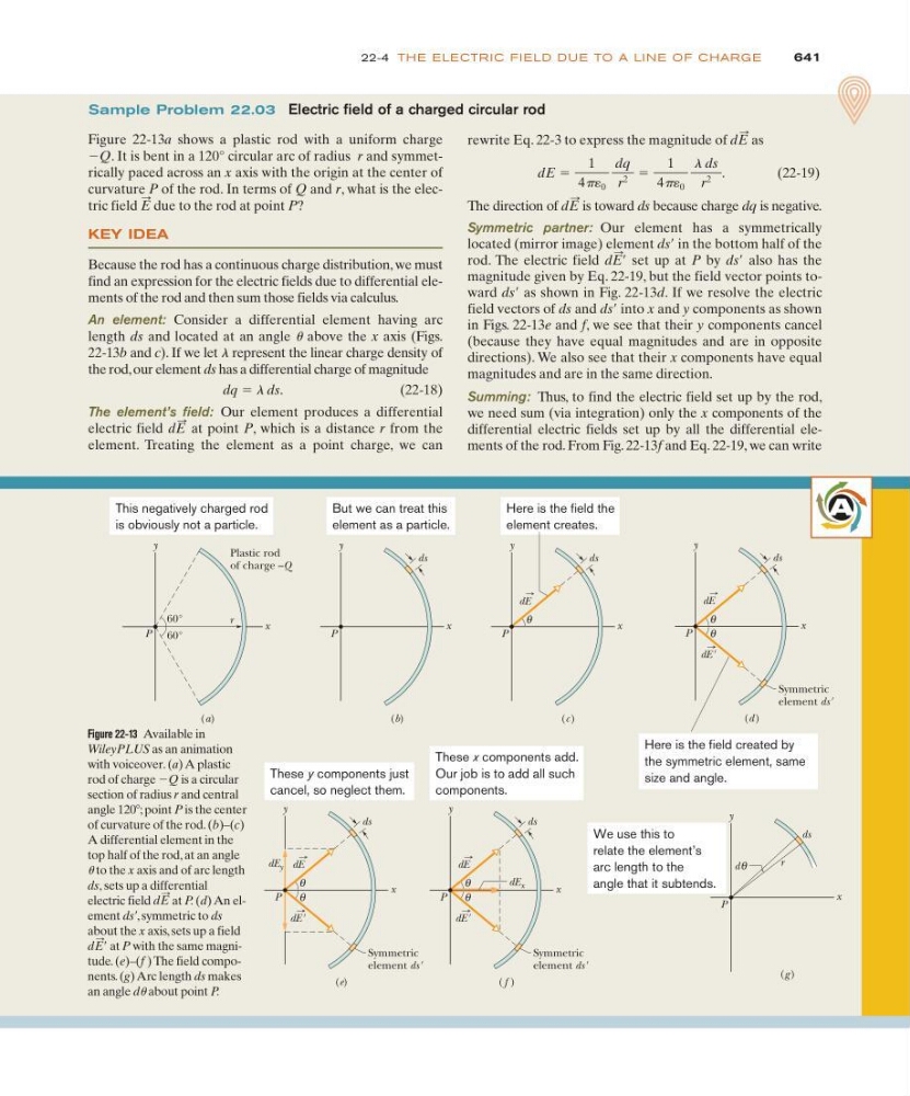
Figure 22-13 Available in
WileyPLUS as an animation
with voiceover. (a) A plastic
rod of charge ϪQ is a circular
section of radius r and central
angle 120Њ; point P is the center
of curvature of the rod. (b)–(c)
A differential element in the
top half of the rod, at an angle
u to the x axis and of arc length
ds, sets up a differential
electric field
at P. (d) An element dsЈ, symmetric to ds
about the x axis, sets up a field
at P with the same magnitude. (e)–(f ) The field components. (g) Arc length ds makes
an angle du about point P.
dE
:
Ј
dE
:
A
Figure 22-13a shows a plastic rod with a uniform charge
ϪQ. It is bent in a 120° circular arc of radius r and symmetrically paced across an x axis with the origin at the center of
curvature P of the rod. In terms of Q and r, what is the electric field due to the rod at point P?
KEY IDEA
Because the rod has a continuous charge distribution, we must
find an expression for the electric fields due to differential elements of the rod and then sum those fields via calculus.
An element: Consider a differential element having arc
length ds and located at an angle u above the x axis (Figs.
22-13b and c). If we let l represent the linear charge density of
the rod, our element ds has a differential charge of magnitude
dq ϭ l ds.
( 2 2 - 1 8 )
The element’s field: Our element produces a differential
electric field
at point P, which is a distance r from the
element. Treating the element as a point charge, we can
dE
:
E
:
rewrite Eq. 22-3 to express the magnitude of
as
(22-19)
The direction of
is toward ds because charge dq is negative.
Symmetric partner: Our element has a symmetrically
located (mirror image) element dsЈ in the bottom half of the
rod. The electric field
set up at P by dsЈ also has the
magnitude given by Eq. 22-19, but the field vector points toward
as shown in Fig. 22-13d. If we resolve the electric
field vectors of ds and
into x and y components as shown
in Figs. 22-13e and f, we see that their y components cancel
(because they have equal magnitudes and are in opposite
directions). We also see that their x components have equal
magnitudes and are in the same direction.
Summing: Thus, to find the electric field set up by the rod,
we need sum (via integration) only the x components of the
differential electric fields set up by all the differential elements of the rod. From Fig. 22-13f and Eq. 22-19, we can write
dsЈ
dsЈ
dE
:
Ј
dE
:
dE ϭ
1
4p´ 0
dq
r
2
ϭ
1
4p´ 0
l ds
r
2
.
dE
: