

Superpixel Segmentation for CC Parcellation in MRI
119
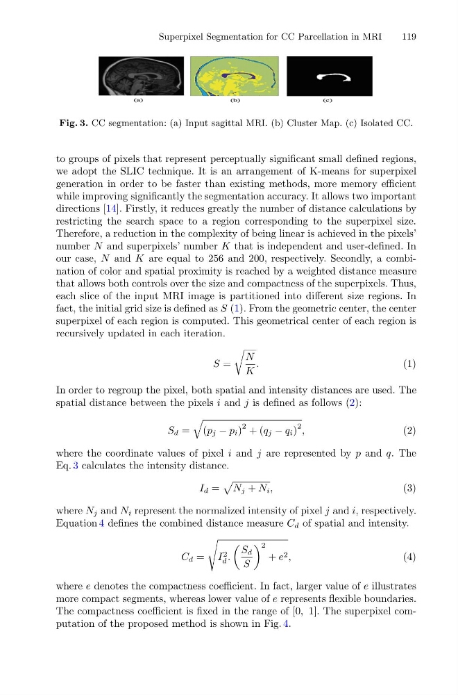
Fig. 3. CC segmentation: (a) Input sagittal MRI. (b) Cluster Map. (c) Isolated CC.
to groups of pixels that represent perceptually significant small defined regions,
we adopt the SLIC technique. It is an arrangement of K-means for superpixel
generation in order to be faster than existing methods, more memory efficient
while improving significantly the segmentation accuracy. It allows two important
directions [14]. Firstly, it reduces greatly the number of distance calculations by
restricting the search space to a region corresponding to the superpixel size.
Therefore, a reduction in the complexity of being linear is achieved in the pixels’
number N and superpixels’ number K that is independent and user-defined. In
our case, N and K are equal to 256 and 200, respectively. Secondly, a combination of color and spatial proximity is reached by a weighted distance measure
that allows both controls over the size and compactness of the superpixels. Thus,
each slice of the input MRI image is partitioned into different size regions. In
fact, the initial grid size is defined as S (1). From the geometric center, the center
superpixel of each region is computed. This geometrical center of each region is
recursively updated in each iteration.
S =
N
K
.
(1)
In order to regroup the pixel, both spatial and intensity distances are used. The
spatial distance between the pixels i and j is defined as follows (2):
S d =
(p j − p i )
2 + (q j − q i )
2 ,
(2)
where the coordinate values of pixel i and j are represented by p and q. The
Eq. 3 calculates the intensity distance.
I d =
N j + N i ,
(3)
where N j and N i represent the normalized intensity of pixel j and i, respectively.
Equation 4 defines the combined distance measure C d of spatial and intensity.
C d =
I 2
d .
S d
S
2
+ e 2 ,
(4)
where e denotes the compactness coefficient. In fact, larger value of e illustrates
more compact segments, whereas lower value of e represents flexible boundaries.
The compactness coefficient is fixed in the range of [0, 1]. The superpixel computation of the proposed method is shown in Fig. 4.
119
Fig. 3. CC segmentation: (a) Input sagittal MRI. (b) Cluster Map. (c) Isolated CC.
to groups of pixels that represent perceptually significant small defined regions,
we adopt the SLIC technique. It is an arrangement of K-means for superpixel
generation in order to be faster than existing methods, more memory efficient
while improving significantly the segmentation accuracy. It allows two important
directions [14]. Firstly, it reduces greatly the number of distance calculations by
restricting the search space to a region corresponding to the superpixel size.
Therefore, a reduction in the complexity of being linear is achieved in the pixels’
number N and superpixels’ number K that is independent and user-defined. In
our case, N and K are equal to 256 and 200, respectively. Secondly, a combination of color and spatial proximity is reached by a weighted distance measure
that allows both controls over the size and compactness of the superpixels. Thus,
each slice of the input MRI image is partitioned into different size regions. In
fact, the initial grid size is defined as S (1). From the geometric center, the center
superpixel of each region is computed. This geometrical center of each region is
recursively updated in each iteration.
S =
N
K
.
(1)
In order to regroup the pixel, both spatial and intensity distances are used. The
spatial distance between the pixels i and j is defined as follows (2):
S d =
(p j − p i )
2 + (q j − q i )
2 ,
(2)
where the coordinate values of pixel i and j are represented by p and q. The
Eq. 3 calculates the intensity distance.
I d =
N j + N i ,
(3)
where N j and N i represent the normalized intensity of pixel j and i, respectively.
Equation 4 defines the combined distance measure C d of spatial and intensity.
C d =
I 2
d .
S d
S
2
+ e 2 ,
(4)
where e denotes the compactness coefficient. In fact, larger value of e illustrates
more compact segments, whereas lower value of e represents flexible boundaries.
The compactness coefficient is fixed in the range of [0, 1]. The superpixel computation of the proposed method is shown in Fig. 4.