

268
8 Solving Ordinary Differential Equations
which differs from u 1 in (8.78) by an amount
1
2 Δt 2 ω 2 u 0 .
Because of the equivalence of (8.76) with the Euler-Cromer scheme, the numerical results will have the same nice properties such as a constant amplitude. There
will be a phase error as in the Euler-Cromer scheme, but this error is effectively
reduced by reducing Δt, as already demonstrated.
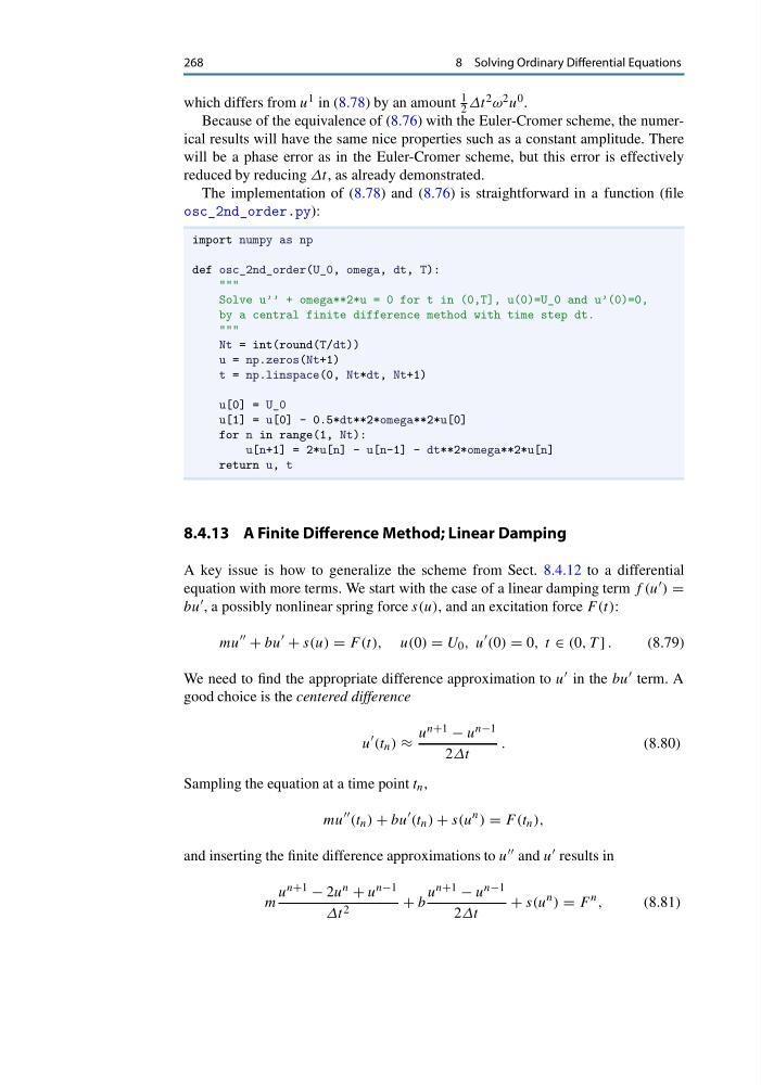
The implementation of (8.78) and (8.76) is straightforward in a function (file
osc_2nd_order.py):
import numpy as np
def osc_2nd_order(U_0, omega, dt, T):
"""
Solve u’’ + omega**2*u = 0 for t in (0,T], u(0)=U_0 and u’(0)=0,
by a central finite difference method with time step dt.
"""
Nt = int(round(T/dt))
u = np.zeros(Nt+1)
t = np.linspace(0, Nt*dt, Nt+1)
u[0] = U_0
u[1] = u[0] - 0.5*dt**2*omega**2*u[0]
for n in range(1, Nt):
u[n+1] = 2*u[n] - u[n-1] - dt**2*omega**2*u[n]
return u, t
8.4.13 A Finite Difference Method; Linear Damping
A key issue is how to generalize the scheme from Sect. 8.4.12 to a differential
equation with more terms. We start with the case of a linear damping term f (u ) =
bu , a possibly nonlinear spring force s(u), and an excitation force F (t):
mu
+ bu
+ s(u) = F (t), u(0) = U 0 , u
(0) = 0, t ∈ (0, T ] .
(8.79)
We need to find the appropriate difference approximation to u in the bu term. A
good choice is the centered difference
u
(t n ) ≈
u n+1 − u n−1
2Δt
.
(8.80)
Sampling the equation at a time point t n ,
mu
(t n ) + bu
(t n ) + s(u
n ) = F (t n ),
and inserting the finite difference approximations to u and u results in
m
u n+1 − 2u n + u n−1
Δt 2
+ b
u n+1 − u n−1
2Δt
+ s(u
n ) = F
n ,
(8.81)
8 Solving Ordinary Differential Equations
which differs from u 1 in (8.78) by an amount
1
2 Δt 2 ω 2 u 0 .
Because of the equivalence of (8.76) with the Euler-Cromer scheme, the numerical results will have the same nice properties such as a constant amplitude. There
will be a phase error as in the Euler-Cromer scheme, but this error is effectively
reduced by reducing Δt, as already demonstrated.
The implementation of (8.78) and (8.76) is straightforward in a function (file
osc_2nd_order.py):
import numpy as np
def osc_2nd_order(U_0, omega, dt, T):
"""
Solve u’’ + omega**2*u = 0 for t in (0,T], u(0)=U_0 and u’(0)=0,
by a central finite difference method with time step dt.
"""
Nt = int(round(T/dt))
u = np.zeros(Nt+1)
t = np.linspace(0, Nt*dt, Nt+1)
u[0] = U_0
u[1] = u[0] - 0.5*dt**2*omega**2*u[0]
for n in range(1, Nt):
u[n+1] = 2*u[n] - u[n-1] - dt**2*omega**2*u[n]
return u, t
8.4.13 A Finite Difference Method; Linear Damping
A key issue is how to generalize the scheme from Sect. 8.4.12 to a differential
equation with more terms. We start with the case of a linear damping term f (u ) =
bu , a possibly nonlinear spring force s(u), and an excitation force F (t):
mu
+ bu
+ s(u) = F (t), u(0) = U 0 , u
(0) = 0, t ∈ (0, T ] .
(8.79)
We need to find the appropriate difference approximation to u in the bu term. A
good choice is the centered difference
u
(t n ) ≈
u n+1 − u n−1
2Δt
.
(8.80)
Sampling the equation at a time point t n ,
mu
(t n ) + bu
(t n ) + s(u
n ) = F (t n ),
and inserting the finite difference approximations to u and u results in
m
u n+1 − 2u n + u n−1
Δt 2
+ b
u n+1 − u n−1
2Δt
+ s(u
n ) = F
n ,
(8.81)