

8.4 Oscillating 1D Systems: A Second Order ODE
267
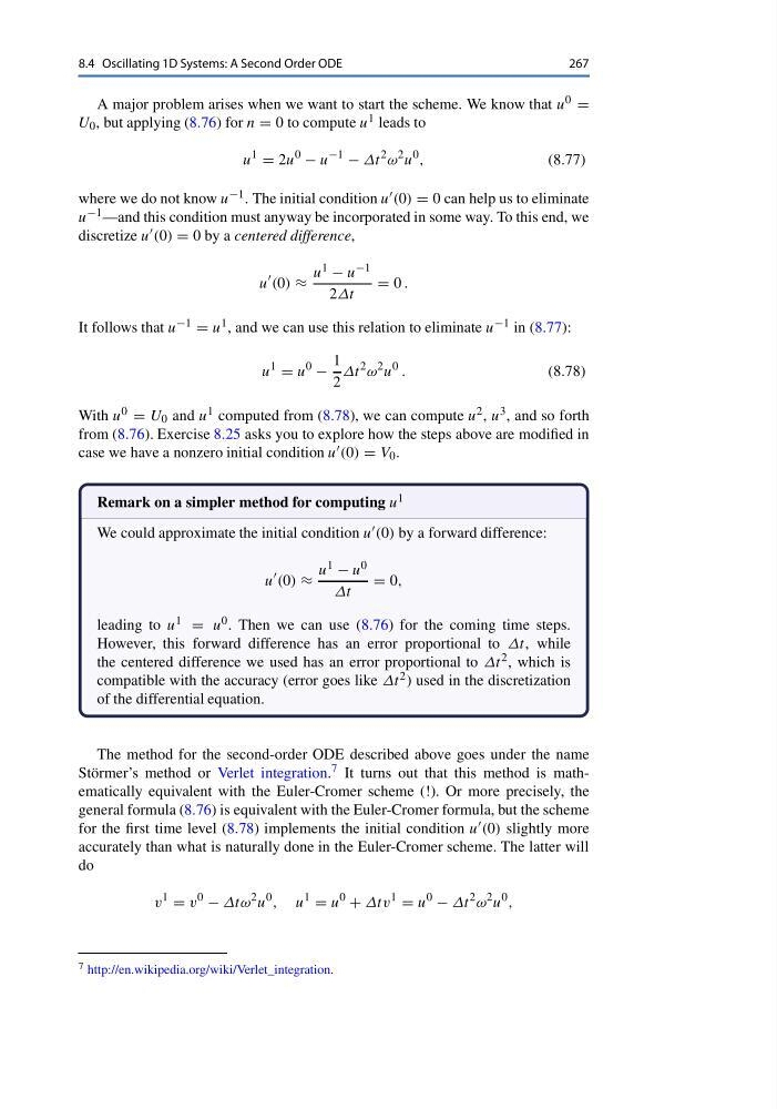
A major problem arises when we want to start the scheme. We know that u 0 =
U 0 , but applying (8.76) for n = 0 to compute u 1 leads to
u
1
= 2u
0
− u
−1
− Δt
2 ω
2 u
0 ,
(8.77)
where we do not know u −1 . The initial condition u (0) = 0 can help us to eliminate
u −1 —and this condition must anyway be incorporated in some way. To this end, we
discretize u (0) = 0 by a centered difference,
u
(0) ≈
u 1 − u −1
2Δt
= 0 .
It follows that u −1 = u 1 , and we can use this relation to eliminate u −1 in (8.77):
u
1
= u
0
−
1
2
Δt
2 ω
2 u
0 .
(8.78)
With u 0 = U 0 and u 1 computed from (8.78), we can compute u 2 , u 3 , and so forth
from (8.76). Exercise 8.25 asks you to explore how the steps above are modified in
case we have a nonzero initial condition u (0) = V 0 .
Remark on a simpler method for computing u 1
We could approximate the initial condition u (0) by a forward difference:
u
(0) ≈
u 1 − u 0
Δt
= 0,
leading to u 1 = u 0 . Then we can use (8.76) for the coming time steps.
However, this forward difference has an error proportional to Δt, while
the centered difference we used has an error proportional to Δt 2 , which is
compatible with the accuracy (error goes like Δt 2 ) used in the discretization
of the differential equation.
The method for the second-order ODE described above goes under the name
Störmer’s method or Verlet integration. 7 It turns out that this method is mathematically equivalent with the Euler-Cromer scheme (!). Or more precisely, the
general formula (8.76) is equivalent with the Euler-Cromer formula, but the scheme
for the first time level (8.78) implements the initial condition u (0) slightly more
accurately than what is naturally done in the Euler-Cromer scheme. The latter will
do
v
1
= v
0
− Δtω
2 u
0 , u
1
= u
0
+ Δtv
1
= u
0
− Δt
2 ω
2 u
0 ,
7 http://en.wikipedia.org/wiki/Verlet_integration.
267
A major problem arises when we want to start the scheme. We know that u 0 =
U 0 , but applying (8.76) for n = 0 to compute u 1 leads to
u
1
= 2u
0
− u
−1
− Δt
2 ω
2 u
0 ,
(8.77)
where we do not know u −1 . The initial condition u (0) = 0 can help us to eliminate
u −1 —and this condition must anyway be incorporated in some way. To this end, we
discretize u (0) = 0 by a centered difference,
u
(0) ≈
u 1 − u −1
2Δt
= 0 .
It follows that u −1 = u 1 , and we can use this relation to eliminate u −1 in (8.77):
u
1
= u
0
−
1
2
Δt
2 ω
2 u
0 .
(8.78)
With u 0 = U 0 and u 1 computed from (8.78), we can compute u 2 , u 3 , and so forth
from (8.76). Exercise 8.25 asks you to explore how the steps above are modified in
case we have a nonzero initial condition u (0) = V 0 .
Remark on a simpler method for computing u 1
We could approximate the initial condition u (0) by a forward difference:
u
(0) ≈
u 1 − u 0
Δt
= 0,
leading to u 1 = u 0 . Then we can use (8.76) for the coming time steps.
However, this forward difference has an error proportional to Δt, while
the centered difference we used has an error proportional to Δt 2 , which is
compatible with the accuracy (error goes like Δt 2 ) used in the discretization
of the differential equation.
The method for the second-order ODE described above goes under the name
Störmer’s method or Verlet integration. 7 It turns out that this method is mathematically equivalent with the Euler-Cromer scheme (!). Or more precisely, the
general formula (8.76) is equivalent with the Euler-Cromer formula, but the scheme
for the first time level (8.78) implements the initial condition u (0) slightly more
accurately than what is naturally done in the Euler-Cromer scheme. The latter will
do
v
1
= v
0
− Δtω
2 u
0 , u
1
= u
0
+ Δtv
1
= u
0
− Δt
2 ω
2 u
0 ,
7 http://en.wikipedia.org/wiki/Verlet_integration.