

266
8 Solving Ordinary Differential Equations
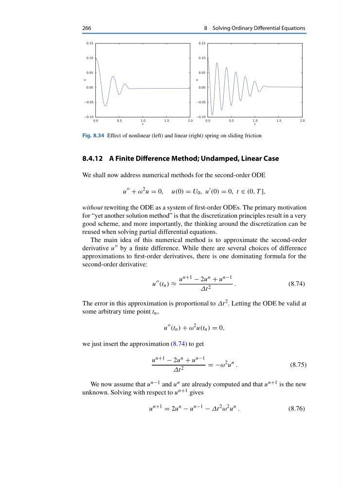
Fig. 8.34 Effect of nonlinear (left) and linear (right) spring on sliding friction
8.4.12 A Finite Difference Method; Undamped, Linear Case
We shall now address numerical methods for the second-order ODE
u
+ ω
2 u = 0, u(0) = U 0 , u
(0) = 0, t ∈ (0, T ],
without rewriting the ODE as a system of first-order ODEs. The primary motivation
for “yet another solution method” is that the discretization principles result in a very
good scheme, and more importantly, the thinking around the discretization can be
reused when solving partial differential equations.
The main idea of this numerical method is to approximate the second-order
derivative u by a finite difference. While there are several choices of difference
approximations to first-order derivatives, there is one dominating formula for the
second-order derivative:
u
(t n ) ≈
u n+1 − 2u n + u n−1
Δt 2
.
(8.74)
The error in this approximation is proportional to Δt 2 . Letting the ODE be valid at
some arbitrary time point t n ,
u
(t n ) + ω
2 u(t n ) = 0,
we just insert the approximation (8.74) to get
u n+1 − 2u n + u n−1
Δt 2
= −ω
2 u
n .
(8.75)
We now assume that u n−1 and u n are already computed and that u n+1 is the new
unknown. Solving with respect to u n+1 gives
u
n+1
= 2u
n
− u
n−1
− Δt
2 ω
2 u
n .
(8.76)
8 Solving Ordinary Differential Equations
Fig. 8.34 Effect of nonlinear (left) and linear (right) spring on sliding friction
8.4.12 A Finite Difference Method; Undamped, Linear Case
We shall now address numerical methods for the second-order ODE
u
+ ω
2 u = 0, u(0) = U 0 , u
(0) = 0, t ∈ (0, T ],
without rewriting the ODE as a system of first-order ODEs. The primary motivation
for “yet another solution method” is that the discretization principles result in a very
good scheme, and more importantly, the thinking around the discretization can be
reused when solving partial differential equations.
The main idea of this numerical method is to approximate the second-order
derivative u by a finite difference. While there are several choices of difference
approximations to first-order derivatives, there is one dominating formula for the
second-order derivative:
u
(t n ) ≈
u n+1 − 2u n + u n−1
Δt 2
.
(8.74)
The error in this approximation is proportional to Δt 2 . Letting the ODE be valid at
some arbitrary time point t n ,
u
(t n ) + ω
2 u(t n ) = 0,
we just insert the approximation (8.74) to get
u n+1 − 2u n + u n−1
Δt 2
= −ω
2 u
n .
(8.75)
We now assume that u n−1 and u n are already computed and that u n+1 is the new
unknown. Solving with respect to u n+1 gives
u
n+1
= 2u
n
− u
n−1
− Δt
2 ω
2 u
n .
(8.76)