

8.5 Rate of Convergence
269
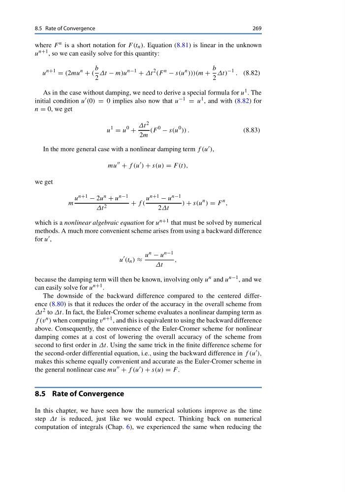
where F n is a short notation for F (t n ). Equation (8.81) is linear in the unknown
u n+1 , so we can easily solve for this quantity:
u
n+1
= (2mu
n
+ (
b
2
Δt − m)u
n−1
+ Δt
2 (F
n
− s(u
n )))(m +
b
2
Δt)
−1 . (8.82)
As in the case without damping, we need to derive a special formula for u 1 . The
initial condition u (0) = 0 implies also now that u −1 = u 1 , and with (8.82) for
n = 0, we get
u
1
= u
0
+
Δt 2
2m
(F
0
− s(u
0 )) .
(8.83)
In the more general case with a nonlinear damping term f (u ),
mu
+ f (u
) + s(u) = F (t),
we get
m
u n+1 − 2u n + u n−1
Δt 2
+ f (
u n+1 − u n−1
2Δt
) + s(u
n ) = F
n ,
which is a nonlinear algebraic equation for u n+1 that must be solved by numerical
methods. A much more convenient scheme arises from using a backward difference
for u ,
u
(t n ) ≈
u n − u n−1
Δt
,
because the damping term will then be known, involving only u n and u n−1 , and we
can easily solve for u n+1 .
The downside of the backward difference compared to the centered difference (8.80) is that it reduces the order of the accuracy in the overall scheme from
Δt 2 to Δt. In fact, the Euler-Cromer scheme evaluates a nonlinear damping term as
f (v n ) when computing v n+1 , and this is equivalent to using the backward difference
above. Consequently, the convenience of the Euler-Cromer scheme for nonlinear
damping comes at a cost of lowering the overall accuracy of the scheme from
second to first order in Δt. Using the same trick in the finite difference scheme for
the second-order differential equation, i.e., using the backward difference in f (u ),
makes this scheme equally convenient and accurate as the Euler-Cromer scheme in
the general nonlinear case mu + f (u ) + s(u) = F .
8.5 Rate of Convergence
In this chapter, we have seen how the numerical solutions improve as the time
step Δt is reduced, just like we would expect. Thinking back on numerical
computation of integrals (Chap. 6), we experienced the same when reducing the
269
where F n is a short notation for F (t n ). Equation (8.81) is linear in the unknown
u n+1 , so we can easily solve for this quantity:
u
n+1
= (2mu
n
+ (
b
2
Δt − m)u
n−1
+ Δt
2 (F
n
− s(u
n )))(m +
b
2
Δt)
−1 . (8.82)
As in the case without damping, we need to derive a special formula for u 1 . The
initial condition u (0) = 0 implies also now that u −1 = u 1 , and with (8.82) for
n = 0, we get
u
1
= u
0
+
Δt 2
2m
(F
0
− s(u
0 )) .
(8.83)
In the more general case with a nonlinear damping term f (u ),
mu
+ f (u
) + s(u) = F (t),
we get
m
u n+1 − 2u n + u n−1
Δt 2
+ f (
u n+1 − u n−1
2Δt
) + s(u
n ) = F
n ,
which is a nonlinear algebraic equation for u n+1 that must be solved by numerical
methods. A much more convenient scheme arises from using a backward difference
for u ,
u
(t n ) ≈
u n − u n−1
Δt
,
because the damping term will then be known, involving only u n and u n−1 , and we
can easily solve for u n+1 .
The downside of the backward difference compared to the centered difference (8.80) is that it reduces the order of the accuracy in the overall scheme from
Δt 2 to Δt. In fact, the Euler-Cromer scheme evaluates a nonlinear damping term as
f (v n ) when computing v n+1 , and this is equivalent to using the backward difference
above. Consequently, the convenience of the Euler-Cromer scheme for nonlinear
damping comes at a cost of lowering the overall accuracy of the scheme from
second to first order in Δt. Using the same trick in the finite difference scheme for
the second-order differential equation, i.e., using the backward difference in f (u ),
makes this scheme equally convenient and accurate as the Euler-Cromer scheme in
the general nonlinear case mu + f (u ) + s(u) = F .
8.5 Rate of Convergence
In this chapter, we have seen how the numerical solutions improve as the time
step Δt is reduced, just like we would expect. Thinking back on numerical
computation of integrals (Chap. 6), we experienced the same when reducing the