

8.4 Oscillating 1D Systems: A Second Order ODE
255
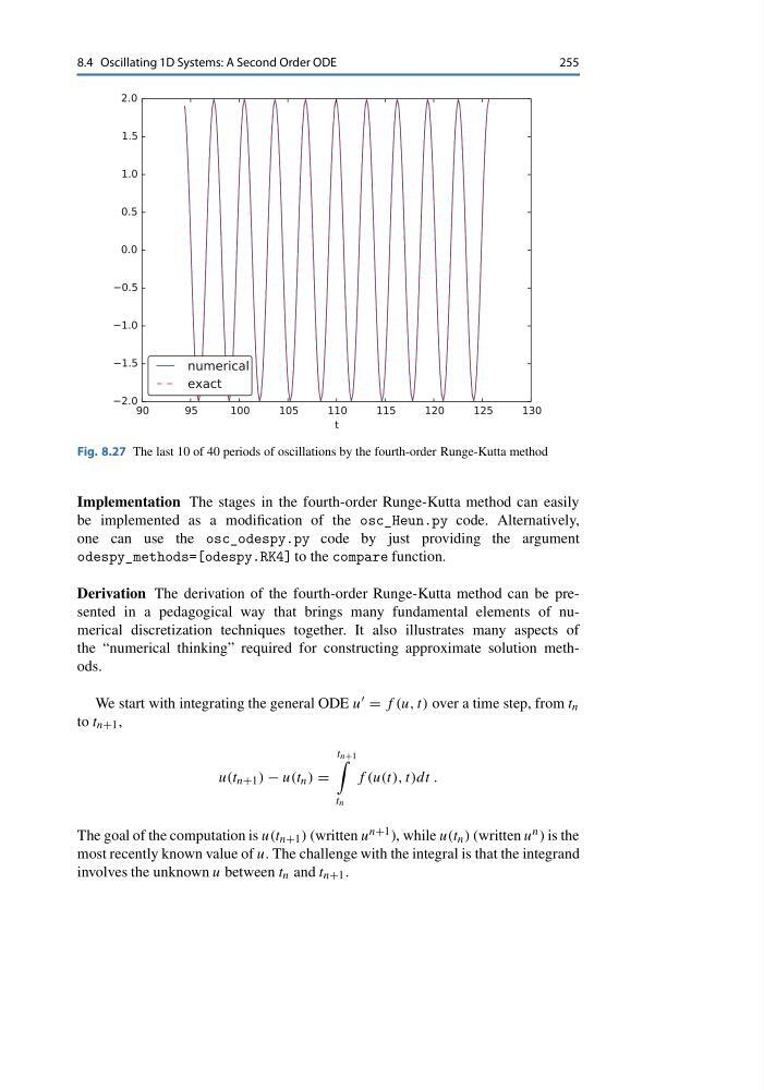
Fig. 8.27 The last 10 of 40 periods of oscillations by the fourth-order Runge-Kutta method
Implementation The stages in the fourth-order Runge-Kutta method can easily
be implemented as a modification of the osc_Heun.py code. Alternatively,
one can use the osc_odespy.py code by just providing the argument
odespy_methods=[odespy.RK4] to the compare function.
Derivation The derivation of the fourth-order Runge-Kutta method can be presented in a pedagogical way that brings many fundamental elements of numerical discretization techniques together. It also illustrates many aspects of
the “numerical thinking” required for constructing approximate solution methods.
We start with integrating the general ODE u = f (u, t) over a time step, from t n
to t n+1 ,
u(t n+1 ) − u(t n ) =
t n+1
t n
f (u(t), t)dt .
The goal of the computation is u(t n+1 ) (written u n+1 ), while u(t n ) (written u n ) is the
most recently known value of u. The challenge with the integral is that the integrand
involves the unknown u between t n and t n+1 .
255
Fig. 8.27 The last 10 of 40 periods of oscillations by the fourth-order Runge-Kutta method
Implementation The stages in the fourth-order Runge-Kutta method can easily
be implemented as a modification of the osc_Heun.py code. Alternatively,
one can use the osc_odespy.py code by just providing the argument
odespy_methods=[odespy.RK4] to the compare function.
Derivation The derivation of the fourth-order Runge-Kutta method can be presented in a pedagogical way that brings many fundamental elements of numerical discretization techniques together. It also illustrates many aspects of
the “numerical thinking” required for constructing approximate solution methods.
We start with integrating the general ODE u = f (u, t) over a time step, from t n
to t n+1 ,
u(t n+1 ) − u(t n ) =
t n+1
t n
f (u(t), t)dt .
The goal of the computation is u(t n+1 ) (written u n+1 ), while u(t n ) (written u n ) is the
most recently known value of u. The challenge with the integral is that the integrand
involves the unknown u between t n and t n+1 .