

256
8 Solving Ordinary Differential Equations
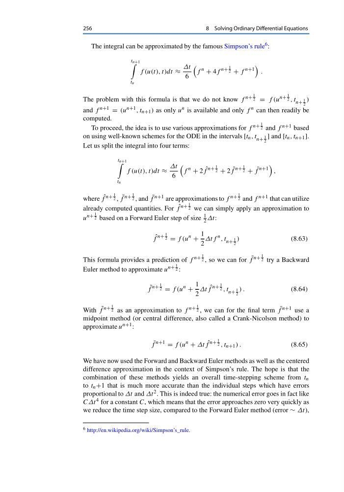
The integral can be approximated by the famous Simpson’s rule 6 :
t n+1
t n
f (u(t), t)dt ≈
Δt
6
f
n
+ 4f
n+
1
2 + f
n+1
.
The problem with this formula is that we do not know f
n+
1
2 = f (u
n+
1
2 , t n+
1
2
)
and f n+1 = (u n+1 , t n+1 ) as only u n is available and only f n can then readily be
computed.
To proceed, the idea is to use various approximations for f
n+
1
2 and f n+1 based
on using well-known schemes for the ODE in the intervals [t n , t n+
1
2
] and [t n , t n+1 ].
Let us split the integral into four terms:
t n+1
t n
f (u(t), t)dt ≈
Δt
6
f
n
+ 2 ˆ
f
n+
1
2 + 2 ˜
f
n+
1
2 + ¯
f
n+1
,
where ˆ
f n+
1
2 , ˜
f n+
1
2 , and ¯
f n+1 are approximations to f n+
1
2 and f n+1 that can utilize
already computed quantities. For ˆ
f
n+
1
2 we can simply apply an approximation to
u
n+
1
2 based on a Forward Euler step of size
1
2 Δt:
ˆ
f
n+
1
2 = f (u
n
+
1
2
Δtf
n , t n+
1
2
)
(8.63)
This formula provides a prediction of f
n+
1
2 , so we can for ˜
f
n+
1
2 try a Backward
Euler method to approximate u
n+
1
2 :
˜
f
n+
1
2 = f (u
n
+
1
2
Δt ˆ
f
n+
1
2 , t n+
1
2
) .
(8.64)
With ˜
f
n+
1
2 as an approximation to f
n+
1
2 , we can for the final term ¯
f n+1 use a
midpoint method (or central difference, also called a Crank-Nicolson method) to
approximate u n+1 :
¯
f
n+1
= f (u
n
+ Δt ˆ
f
n+
1
2 , t n+1 ) .
(8.65)
We have now used the Forward and Backward Euler methods as well as the centered
difference approximation in the context of Simpson’s rule. The hope is that the
combination of these methods yields an overall time-stepping scheme from t n
to t n +1 that is much more accurate than the individual steps which have errors
proportional to Δt and Δt 2 . This is indeed true: the numerical error goes in fact like
CΔt 4 for a constant C, which means that the error approaches zero very quickly as
we reduce the time step size, compared to the Forward Euler method (error ∼ Δt),
6 http://en.wikipedia.org/wiki/Simpson’s_rule.
8 Solving Ordinary Differential Equations
The integral can be approximated by the famous Simpson’s rule 6 :
t n+1
t n
f (u(t), t)dt ≈
Δt
6
f
n
+ 4f
n+
1
2 + f
n+1
.
The problem with this formula is that we do not know f
n+
1
2 = f (u
n+
1
2 , t n+
1
2
)
and f n+1 = (u n+1 , t n+1 ) as only u n is available and only f n can then readily be
computed.
To proceed, the idea is to use various approximations for f
n+
1
2 and f n+1 based
on using well-known schemes for the ODE in the intervals [t n , t n+
1
2
] and [t n , t n+1 ].
Let us split the integral into four terms:
t n+1
t n
f (u(t), t)dt ≈
Δt
6
f
n
+ 2 ˆ
f
n+
1
2 + 2 ˜
f
n+
1
2 + ¯
f
n+1
,
where ˆ
f n+
1
2 , ˜
f n+
1
2 , and ¯
f n+1 are approximations to f n+
1
2 and f n+1 that can utilize
already computed quantities. For ˆ
f
n+
1
2 we can simply apply an approximation to
u
n+
1
2 based on a Forward Euler step of size
1
2 Δt:
ˆ
f
n+
1
2 = f (u
n
+
1
2
Δtf
n , t n+
1
2
)
(8.63)
This formula provides a prediction of f
n+
1
2 , so we can for ˜
f
n+
1
2 try a Backward
Euler method to approximate u
n+
1
2 :
˜
f
n+
1
2 = f (u
n
+
1
2
Δt ˆ
f
n+
1
2 , t n+
1
2
) .
(8.64)
With ˜
f
n+
1
2 as an approximation to f
n+
1
2 , we can for the final term ¯
f n+1 use a
midpoint method (or central difference, also called a Crank-Nicolson method) to
approximate u n+1 :
¯
f
n+1
= f (u
n
+ Δt ˆ
f
n+
1
2 , t n+1 ) .
(8.65)
We have now used the Forward and Backward Euler methods as well as the centered
difference approximation in the context of Simpson’s rule. The hope is that the
combination of these methods yields an overall time-stepping scheme from t n
to t n +1 that is much more accurate than the individual steps which have errors
proportional to Δt and Δt 2 . This is indeed true: the numerical error goes in fact like
CΔt 4 for a constant C, which means that the error approaches zero very quickly as
we reduce the time step size, compared to the Forward Euler method (error ∼ Δt),
6 http://en.wikipedia.org/wiki/Simpson’s_rule.