

254
8 Solving Ordinary Differential Equations
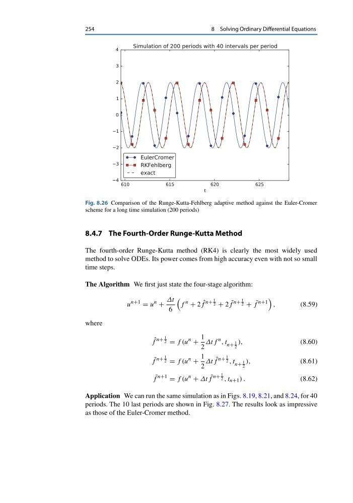
Fig. 8.26 Comparison of the Runge-Kutta-Fehlberg adaptive method against the Euler-Cromer
scheme for a long time simulation (200 periods)
8.4.7 The Fourth-Order Runge-Kutta Method
The fourth-order Runge-Kutta method (RK4) is clearly the most widely used
method to solve ODEs. Its power comes from high accuracy even with not so small
time steps.
The Algorithm We first just state the four-stage algorithm:
u
n+1
= u
n
+
Δt
6
f
n
+ 2 ˆ
f
n+
1
2 + 2 ˜
f
n+
1
2 + ¯
f
n+1
,
(8.59)
where
ˆ
f
n+
1
2 = f (u
n
+
1
2
Δtf
n , t n+
1
2
),
(8.60)
˜
f
n+
1
2 = f (u
n
+
1
2
Δt ˆ
f
n+
1
2 , t n+
1
2
),
(8.61)
¯
f
n+1
= f (u
n
+ Δt ˜
f
n+
1
2 , t n+1 ) .
(8.62)
Application We can run the same simulation as in Figs. 8.19, 8.21, and 8.24, for 40
periods. The 10 last periods are shown in Fig. 8.27. The results look as impressive
as those of the Euler-Cromer method.
8 Solving Ordinary Differential Equations
Fig. 8.26 Comparison of the Runge-Kutta-Fehlberg adaptive method against the Euler-Cromer
scheme for a long time simulation (200 periods)
8.4.7 The Fourth-Order Runge-Kutta Method
The fourth-order Runge-Kutta method (RK4) is clearly the most widely used
method to solve ODEs. Its power comes from high accuracy even with not so small
time steps.
The Algorithm We first just state the four-stage algorithm:
u
n+1
= u
n
+
Δt
6
f
n
+ 2 ˆ
f
n+
1
2 + 2 ˜
f
n+
1
2 + ¯
f
n+1
,
(8.59)
where
ˆ
f
n+
1
2 = f (u
n
+
1
2
Δtf
n , t n+
1
2
),
(8.60)
˜
f
n+
1
2 = f (u
n
+
1
2
Δt ˆ
f
n+
1
2 , t n+
1
2
),
(8.61)
¯
f
n+1
= f (u
n
+ Δt ˜
f
n+
1
2 , t n+1 ) .
(8.62)
Application We can run the same simulation as in Figs. 8.19, 8.21, and 8.24, for 40
periods. The 10 last periods are shown in Fig. 8.27. The results look as impressive
as those of the Euler-Cromer method.