

8.4 Oscillating 1D Systems: A Second Order ODE
253
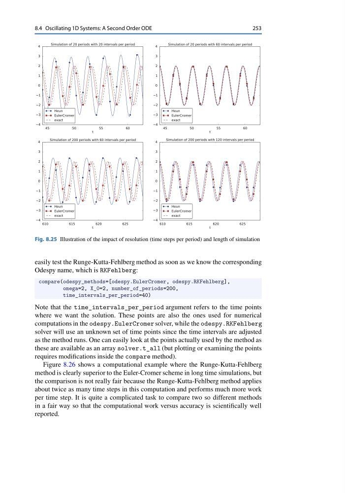
Fig. 8.25 Illustration of the impact of resolution (time steps per period) and length of simulation
easily test the Runge-Kutta-Fehlberg method as soon as we know the corresponding
Odespy name, which is RKFehlberg:
compare(odespy_methods=[odespy.EulerCromer, odespy.RKFehlberg],
omega=2, X_0=2, number_of_periods=200,
time_intervals_per_period=40)
Note that the time_intervals_per_period argument refers to the time points
where we want the solution. These points are also the ones used for numerical
computations in the odespy.EulerCromer solver, while the odespy.RKFehlberg
solver will use an unknown set of time points since the time intervals are adjusted
as the method runs. One can easily look at the points actually used by the method as
these are available as an array solver.t_all (but plotting or examining the points
requires modifications inside the compare method).
Figure 8.26 shows a computational example where the Runge-Kutta-Fehlberg
method is clearly superior to the Euler-Cromer scheme in long time simulations, but
the comparison is not really fair because the Runge-Kutta-Fehlberg method applies
about twice as many time steps in this computation and performs much more work
per time step. It is quite a complicated task to compare two so different methods
in a fair way so that the computational work versus accuracy is scientifically well
reported.
253
Fig. 8.25 Illustration of the impact of resolution (time steps per period) and length of simulation
easily test the Runge-Kutta-Fehlberg method as soon as we know the corresponding
Odespy name, which is RKFehlberg:
compare(odespy_methods=[odespy.EulerCromer, odespy.RKFehlberg],
omega=2, X_0=2, number_of_periods=200,
time_intervals_per_period=40)
Note that the time_intervals_per_period argument refers to the time points
where we want the solution. These points are also the ones used for numerical
computations in the odespy.EulerCromer solver, while the odespy.RKFehlberg
solver will use an unknown set of time points since the time intervals are adjusted
as the method runs. One can easily look at the points actually used by the method as
these are available as an array solver.t_all (but plotting or examining the points
requires modifications inside the compare method).
Figure 8.26 shows a computational example where the Runge-Kutta-Fehlberg
method is clearly superior to the Euler-Cromer scheme in long time simulations, but
the comparison is not really fair because the Runge-Kutta-Fehlberg method applies
about twice as many time steps in this computation and performs much more work
per time step. It is quite a complicated task to compare two so different methods
in a fair way so that the computational work versus accuracy is scientifically well
reported.