

252
8 Solving Ordinary Differential Equations
# Compute the time points where we want the solution
N_t = int(round(T/dt))
time_points = np.linspace(0, N_t*dt, N_t+1)
legends = []
for solver in solvers:
sol, t = solver.solve(time_points)
v = sol[:,0]
u = sol[:,1]
# Plot only the last p periods
p = 6
m = p*time_intervals_per_period # no time steps to plot
plt.plot(t[-m:], u[-m:])
plt.hold(’on’)
legends.append(solver.name())
plt.xlabel(’t’)
# Plot exact solution too
plt.plot(t[-m:], X_0*np.cos(omega*t)[-m:], ’k--’)
legends.append(’exact’)
plt.legend(legends, loc=’lower left’)
plt.axis([t[-m], t[-1], -2*X_0, 2*X_0])
plt.title(’Simulation of {:d} periods with {:d} intervals per period’\
.format(number_of_periods, time_intervals_per_period))
plt.savefig(’tmp.pdf’); plt.savefig(’tmp.png’)
plt.show()
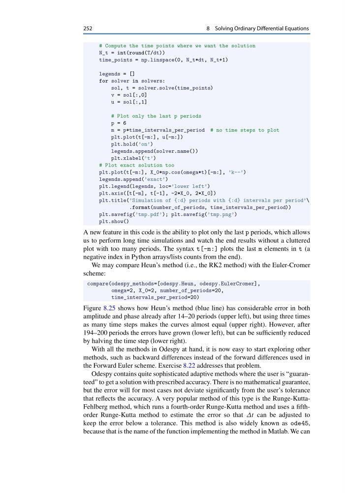
A new feature in this code is the ability to plot only the last p periods, which allows
us to perform long time simulations and watch the end results without a cluttered
plot with too many periods. The syntax t[-m:] plots the last m elements in t (a
negative index in Python arrays/lists counts from the end).
We may compare Heun’s method (i.e., the RK2 method) with the Euler-Cromer
scheme:
compare(odespy_methods=[odespy.Heun, odespy.EulerCromer],
omega=2, X_0=2, number_of_periods=20,
time_intervals_per_period=20)
Figure 8.25 shows how Heun’s method (blue line) has considerable error in both
amplitude and phase already after 14–20 periods (upper left), but using three times
as many time steps makes the curves almost equal (upper right). However, after
194–200 periods the errors have grown (lower left), but can be sufficiently reduced
by halving the time step (lower right).
With all the methods in Odespy at hand, it is now easy to start exploring other
methods, such as backward differences instead of the forward differences used in
the Forward Euler scheme. Exercise 8.22 addresses that problem.
Odespy contains quite sophisticated adaptive methods where the user is “guaranteed” to get a solution with prescribed accuracy. There is no mathematical guarantee,
but the error will for most cases not deviate significantly from the user’s tolerance
that reflects the accuracy. A very popular method of this type is the Runge-KuttaFehlberg method, which runs a fourth-order Runge-Kutta method and uses a fifthorder Runge-Kutta method to estimate the error so that Δt can be adjusted to
keep the error below a tolerance. This method is also widely known as ode45,
because that is the name of the function implementing the method in Matlab. We can
8 Solving Ordinary Differential Equations
# Compute the time points where we want the solution
N_t = int(round(T/dt))
time_points = np.linspace(0, N_t*dt, N_t+1)
legends = []
for solver in solvers:
sol, t = solver.solve(time_points)
v = sol[:,0]
u = sol[:,1]
# Plot only the last p periods
p = 6
m = p*time_intervals_per_period # no time steps to plot
plt.plot(t[-m:], u[-m:])
plt.hold(’on’)
legends.append(solver.name())
plt.xlabel(’t’)
# Plot exact solution too
plt.plot(t[-m:], X_0*np.cos(omega*t)[-m:], ’k--’)
legends.append(’exact’)
plt.legend(legends, loc=’lower left’)
plt.axis([t[-m], t[-1], -2*X_0, 2*X_0])
plt.title(’Simulation of {:d} periods with {:d} intervals per period’\
.format(number_of_periods, time_intervals_per_period))
plt.savefig(’tmp.pdf’); plt.savefig(’tmp.png’)
plt.show()
A new feature in this code is the ability to plot only the last p periods, which allows
us to perform long time simulations and watch the end results without a cluttered
plot with too many periods. The syntax t[-m:] plots the last m elements in t (a
negative index in Python arrays/lists counts from the end).
We may compare Heun’s method (i.e., the RK2 method) with the Euler-Cromer
scheme:
compare(odespy_methods=[odespy.Heun, odespy.EulerCromer],
omega=2, X_0=2, number_of_periods=20,
time_intervals_per_period=20)
Figure 8.25 shows how Heun’s method (blue line) has considerable error in both
amplitude and phase already after 14–20 periods (upper left), but using three times
as many time steps makes the curves almost equal (upper right). However, after
194–200 periods the errors have grown (lower left), but can be sufficiently reduced
by halving the time step (lower right).
With all the methods in Odespy at hand, it is now easy to start exploring other
methods, such as backward differences instead of the forward differences used in
the Forward Euler scheme. Exercise 8.22 addresses that problem.
Odespy contains quite sophisticated adaptive methods where the user is “guaranteed” to get a solution with prescribed accuracy. There is no mathematical guarantee,
but the error will for most cases not deviate significantly from the user’s tolerance
that reflects the accuracy. A very popular method of this type is the Runge-KuttaFehlberg method, which runs a fourth-order Runge-Kutta method and uses a fifthorder Runge-Kutta method to estimate the error so that Δt can be adjusted to
keep the error below a tolerance. This method is also widely known as ode45,
because that is the name of the function implementing the method in Matlab. We can