

246
8 Solving Ordinary Differential Equations
The standard way of expressing this scheme in physics is to change the order of
the equations,
v
= −ω
2 u,
(8.53)
u
= v,
(8.54)
and apply a forward difference to (8.53) and a backward difference to (8.54):
v
n+1
= v
n
− Δt ω
2 u
n ,
(8.55)
u
n+1
= u
n
+ Δt v
n+1 .
(8.56)
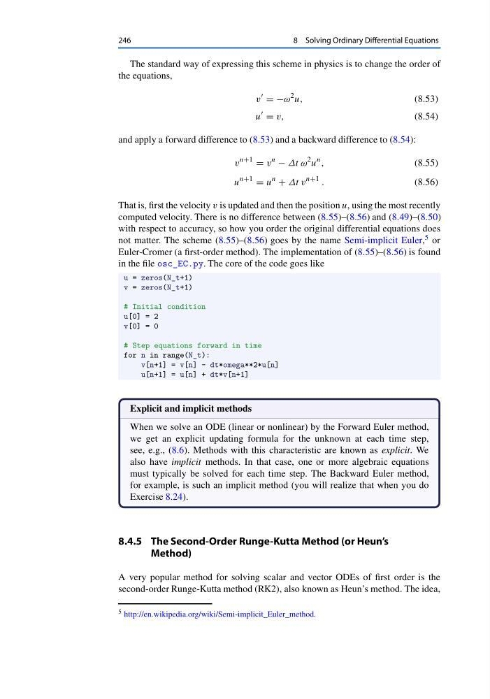
That is, first the velocity v is updated and then the position u, using the most recently
computed velocity. There is no difference between (8.55)–(8.56) and (8.49)–(8.50)
with respect to accuracy, so how you order the original differential equations does
not matter. The scheme (8.55)–(8.56) goes by the name Semi-implicit Euler, 5 or
Euler-Cromer (a first-order method). The implementation of (8.55)–(8.56) is found
in the file osc_EC.py. The core of the code goes like
u = zeros(N_t+1)
v = zeros(N_t+1)
# Initial condition
u[0] = 2
v[0] = 0
# Step equations forward in time
for n in range(N_t):
v[n+1] = v[n] - dt*omega**2*u[n]
u[n+1] = u[n] + dt*v[n+1]
Explicit and implicit methods
When we solve an ODE (linear or nonlinear) by the Forward Euler method,
we get an explicit updating formula for the unknown at each time step,
see, e.g., (8.6). Methods with this characteristic are known as explicit. We
also have implicit methods. In that case, one or more algebraic equations
must typically be solved for each time step. The Backward Euler method,
for example, is such an implicit method (you will realize that when you do
Exercise 8.24).
8.4.5 The Second-Order Runge-Kutta Method (or Heun’s
Method)
A very popular method for solving scalar and vector ODEs of first order is the
second-order Runge-Kutta method (RK2), also known as Heun’s method. The idea,
5 http://en.wikipedia.org/wiki/Semi-implicit_Euler_method.
8 Solving Ordinary Differential Equations
The standard way of expressing this scheme in physics is to change the order of
the equations,
v
= −ω
2 u,
(8.53)
u
= v,
(8.54)
and apply a forward difference to (8.53) and a backward difference to (8.54):
v
n+1
= v
n
− Δt ω
2 u
n ,
(8.55)
u
n+1
= u
n
+ Δt v
n+1 .
(8.56)
That is, first the velocity v is updated and then the position u, using the most recently
computed velocity. There is no difference between (8.55)–(8.56) and (8.49)–(8.50)
with respect to accuracy, so how you order the original differential equations does
not matter. The scheme (8.55)–(8.56) goes by the name Semi-implicit Euler, 5 or
Euler-Cromer (a first-order method). The implementation of (8.55)–(8.56) is found
in the file osc_EC.py. The core of the code goes like
u = zeros(N_t+1)
v = zeros(N_t+1)
# Initial condition
u[0] = 2
v[0] = 0
# Step equations forward in time
for n in range(N_t):
v[n+1] = v[n] - dt*omega**2*u[n]
u[n+1] = u[n] + dt*v[n+1]
Explicit and implicit methods
When we solve an ODE (linear or nonlinear) by the Forward Euler method,
we get an explicit updating formula for the unknown at each time step,
see, e.g., (8.6). Methods with this characteristic are known as explicit. We
also have implicit methods. In that case, one or more algebraic equations
must typically be solved for each time step. The Backward Euler method,
for example, is such an implicit method (you will realize that when you do
Exercise 8.24).
8.4.5 The Second-Order Runge-Kutta Method (or Heun’s
Method)
A very popular method for solving scalar and vector ODEs of first order is the
second-order Runge-Kutta method (RK2), also known as Heun’s method. The idea,
5 http://en.wikipedia.org/wiki/Semi-implicit_Euler_method.